Thursday, March 5, 2026
Home Blog Page 12

Aperiodic signals

0

Aperiodic signals:

If the signal does not repeat at regular intervals of time is called aperiodic signal.
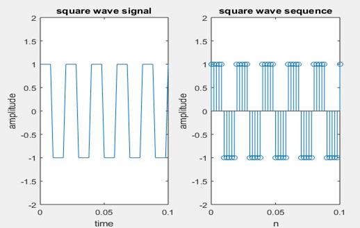
Square wave:

Let us consider an example for square wave in matlab.

clc;

clear all;

close all;

t=0:0.002:0.1;

y=square(2*pi*50*t);

figure;

subplot(1,2,1);

plot(t,y);

axis([0 0.1 -2 2]);

xlabel(‘time’);

ylabel(‘amplitude’);

title(‘square wave signal’);

%generation of square wave sequence

subplot(1,2,2);

stem(t,y);

axis([0 0.1 -2 2]);

xlabel(‘n’);

ylabel(‘amplitude’);

title(‘square wave sequence’);
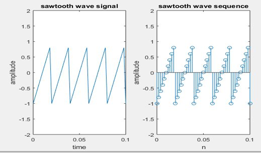
Sawtooth wave:

Let us consider an example of sawtooth wave in matlab.

clc;

clear all;

close all;

%generation of sawtooth signal

t=0:0.002:0.1;

y=sawtooth(2*pi*50*t);

subplot(1,2,1);

plot(t,y);

axis([0 0.1 -2 2]);

xlabel(‘time’);

ylabel(‘amplitude’);

title(‘sawtooth wave signal’);

%generation of sawtooth sequence

subplot(1,2,2);

stem(t,y);

axis([0 0.1 -2 2]);

xlabel(‘n’);

ylabel(‘amplitude’);

title(‘sawtooth wave sequence’);
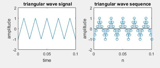
Triangular wave:

Let us consider an example of triangular wave in matlab.

clc;

clear all;

close all;

%generation of triangular wave signal

t=0:0.002:0.1;

y=sawtooth(2*pi*50*t,.5);

figure;

subplot(2,2,1);

plot(t,y);

axis([0 0.1 -2 2]);

xlabel(‘time’);

ylabel(‘amplitude’);

title(‘ triangular wave signal’);

%generation of triangular wave sequence

subplot(2,2,2);

stem(t,y);

axis([0 0.1 -2 2]);

xlabel(‘n’);

ylabel(‘amplitude’);

title(‘triangular wave sequence’);

DATA COMMUNICATION

DATA COMMUNICATION:

If one is communicating means sharing some relevant data these sharing can be local or remote. While sharing information face to face is called as local whereas sharing over some distance is called as remote. The term telecommunication may include telephone, telegraph etc., and communication means at a distance.

And the term data communication determines exchange of information between two devices by using some transmission medium.

Data communication depends upon some basic characteristics:

Delivery:

The term delivery means sending data to the intended destination.

Accuracy:

The system will delivered the data without altering the information to the destination.

Timelines:

Data must delivered to the end device with in a timely manner, if the data is delivered late it will be useless.

Jitter:

Jitter is defined as variation in the packet arrival time. For example if we send a video packet every 30ms. If it is arrive with the delay of 30ms it will result in uneven quality in the video.

Components in data communication:

There are five components in data communication:

Message:

The message is the data to be communicated. Most popular form of message which may include text, pictures, video, audio and numbers.

Sender:

Sender is the equipment that sends the message. Sender may include camera, telephone, computer and workstation and so on.

Receiver:

Receiver is the equipment that receives the information from medium, which may include camera, telephone, computer and workstation and so on.

Transmission medium or physical path:

In information is travelled form sender to receiver via some physical medium, some examples of transmission medium are radio waves, coaxial cables and twisted pair ,so on.

Protocol:

A protocol is defined as an agreement between communicating devices, without protocol the communication cannot be done connection of two devices may be done.

GENERATION OF SIGNALS AND SEQUENCES

0

GENERATION OF SIGNALS AND SEQUENCES:

If we defines amplitude of the signal at every instant of time is called continuous time signal, else if we define at some instant of time is called discrete time signal. If the signal repeats at regular intervals is called as periodic signal. Else it is called as aperiodic. Let us consider some example of periodic and aperiodic signals.

Periodic: ramp, sinc, unit step and ramp.

Aperiodic: sawtooth, square, triangular sinusoidal.

Ramp signal:

The ramp function is a singular real function.it is applied in engineering. Easily computable because of the mean of the experimental variable and its definite quantity. Ramp function is defined as:

               r(t)= t   when   t≥0

0 Otherwise

clc;

clear all;

close all;

t=0:0.001:0.1;

y1=t;

figure;

subplot(2,2,1);

plot(t,y1);

xlabel(‘time’);

ylabel(‘amplitude’);

title(‘ramp signal’);

%generation of ramp sequence

subplot(2,2,2);

stem(t,y1);

xlabel(‘n’);

ylabel(‘amplitude’);

title(‘ramp sequence’);

Unit step:

Unit step function is considered as a fundamental function in engineering and strongly recommended which the reader becomes very familiar.

u(t) =0 if t<0

         1 if t>0

          ½ if t=0

clc;

clear all;

close all;

t=-12:1:12;

y=(t>=0);

subplot(2,2,1);

plot(t,y);

xlabel(‘time’);

ylabel(‘amplitude’);

title(‘unit step signal’);

%generation of unit step sequence

subplot(2,2,2);

stem(t,y);

xlabel(‘n’);

ylabel(‘amplitude’);

title(‘unit step sequence’);

Unit impulse:

Unit impulse function is most useful function in study of linear system.

S(t) =1 when t=0

         0 otherwise

clc;

clear all;

close all;

%generation of unit impulse signal

t1=-1:0.01:1

y1=(t1==0);

subplot(2,2,1);

plot(t1,y1);

xlabel(‘time’);

ylabel(‘amplitude’);

title(‘unit impulse signal’);

%generation of impulse sequence

subplot(2,2,2);

stem(t1,y1);

xlabel(‘n’);

ylabel(‘amplitude’);

title(‘unit impulse sequence’);

Types of Production Systems

 The following are the types of production systems.

Forward Production Systems:

  1. A Production system in which starting from an initial state moving towards the goal state is termed as Forward Production Systems.

Backward Production Systems:

  1. A Production system in which starting at goal state and tracing back towards initial state.

Specialized production systems:

 There are two types of Specialized Production systems they are

  1. Commutative production system
  2. Decomposable Production System

Commutative production system:

A production system is said to be commutative if it satisfies the following property

  1. Each member of set of rules applicable to D is also applicable to any database produced by applying an applicable rule to ‘D’
  2. If the goal condition is satisfied by ‘D’ then it is also satisfied by any data base produced by applying any applicable rule to ’D’.
  3. The database that results by applying to ‘D’ any sequence composed of rules that are application to D is invariant under permutations of the sequence.

Overall computation cost of AI Production System, Types of Control Strategy

Overall computation cost of AI Production System:

 Rule application cost and control strategy cost together constitutes to the over all computation cost of AI production system.

For an efficient AI system to design there must be balancing between the rule application cost and control strategy.

An efficient AI system involves the usage of the techniques that uses large amount of problem related information without acquiring excessive  control cost.

Types of Control Strategy

There are two types of control strategy they are

  1. Irrevocable
  2. Tentative
  3. Backtracking
  4. Graph Search Control

Irrevocable Strategy:

It is a type of control strategy in which once the rule is applied it cannot be retraced.

Here in this, the applicable rule is applied without any provision for reconsideration.

Tentative Strategy:

App rule is applied but provision is made to return later to this point in the computation to apply some other rule. Tentative strategy includes:

Backtracking:

 In this a point is established to which the state of communication can revert to this point.

 In this, there is a provision that  is made for monitoring the effects of several sequences of rules simultaneously.

Procedure for production, Computational Cost, Control Strategy cost

Procedure for production

Initially we have a data base that has updated data and we continue to work with operators till we reach a goal condition.

We select  some  rule’ R’ from the set of rules applied to the data.

We apply that rule to generate new data.

We continually perform this until we reach the required condition.

If the required condition is achieved then we say that the problem is achieved.

Control Strategy 

Selecting the rules and keeping track of those sequence of rules and the database they produce constitute is termed as control strategy for production system.

Operations of AI production systems can be characterized as a search process in which rules are tried until some sequence of them is found that produces a database satisfying the termination condition.

Computational Cost

 Very important attribute for selecting rules is the amount of information that you aware of   about the problem.

In the worst case if I don’t know any thing about the problem the rule can be selected arbitrarily, as I don’t know anything about the problem.

 At the informed extreme , when I know the complete knowledge about the problem  the control strategy is guided by the problem knowledge and this  guidance is enough to select  a correct rule every time.

Overall computational cost of  a AI production system can be categorized into two  major categories.

Rule Application Cost:

For uninformed Control System:

In this system we have try a large number of rules to find a solution ,Therefore we have a high rule application cost.

For informed Control System:

In informed control system the production system is directly guided to the solution, Therefore very less Rule Application Cost

Control Strategy Cost:

For uninformed Control System:

Here in this case  arbitrary selection does not depend on costly computation. Therefore we have a low computational Cost.

For informed Control System:

To inform about the problem domain, cost in terms of storage and computation. Therefore we have a high control strategy computation.

Operations of AI production system: Introduction to Control strategy, Production system Vs Conventional Computation

Operations of AI production system

The operation of AI production system can thus be characterized  as a search process in which rules are tried until some sequence of them is found. To solve a problem using a production system we must specify the database Rules

Control Strategy

Converting a problem statement into the above three components of a production system is the problem  representation in AI. Once this is successfully done we only have problem solving which is just about searching in that problem space for the given goal state given the initial state.

A production system consists of productions (rules), a working memory of facts (database) and   Control strategy is about an algorithm for producing new facts from old. As we have seen in the 8 puzzle example a rule becomes eligible to fire when its conditions match  some set of elements currently in the working memory. As it matches left side the rule is fired and we have new facts, which is the facts that are generated on the right side of the rule.

A control strategy determines which of the several eligible rules fires next. It is important to realize   the difference within production system and conventional computation.

Production System Versus Conventional Computation

 Though both the systems use hierarchically organized programs, they have many differences .Irrespective of any local database, global database is accessible for everyone..

Here the communication takes place only between the databases but not between the rules.

Production system structure is modular; changes to any of the components made independently.

Using Conventional Computation in AI application is difficult, For any change in knowledge base would require extensive changes to the program

Inverse Laplace Transform

0

Ilaplace command used to perform the inverse laplace transform for the given function. Let us consider an example;

F(s) =


F= 5*(s+2)/(s*(s^2+9*s+5));

 ilaplace (F)

ans = 9*exp(-2*t)*cos(t)+3 *exp(-2*t)*sin(t)+5

In inverse laplace transform function hyperbolic expression can solved

Sinh(x)=

Cosh(x)=

Fourier Transform In Matlab:

Some numerical methods are used for solving continuous time signals in matlab with Fourier transform. Let us choose an example to plot fourier transform function

f=-6:.01:6;

 X=9*sinc(9*f);

 plot(f,X)

Fast Fourier Transform:

Depending on the length of the sequence being transformed with the DFT the computation of this transform are often time consuming. The Fast Fourier Transform (FFT) is an algorithm for computing the DFT of a sequence during a more efficient manner. MATLAB provides a inbuilt command for computing the FFT of a sequence.

For example, using the same two-frequency signal x(t) used above we can produce a sequence of samples of length N = 150 spaced every Ts = .0003 seconds as shown previously.

Whilethe frequency components are spaced every 1/(N*Ts) Hz and the corresponding frequency values  are from 0 to (N-1)/(N*Ts) Hz as shown below.

In order to plot a fast fourier transform (fft) by using fft command

clear

 N=150;

 ts=.0003;

 deltaf=1/(N*ts);

 t=[0:N-1]*ts;

 x=cos(2*pi*100*t)+cos(2*pi*500*t);

 Xf=fft(x);

 f=[0:N-1]*deltaf;

 plot (f,abs(Xf)

In order to plot a fast fourier transform (fft) we should follow two rules

In order to plot a fast fourier transform (fft) we should follow two rules
Select Ts as large as possible but in order that the very best frequency component in your signal is a smaller amount than 1/2Ts. 2.

After determining the worth of Ts, select N in order that 1/NTs, the frequency resolution is little enough to accurately display your frequency components.

INTEGRATION IN MATLAB

0

INTEGRATION IN MATLAB

Integration will solve two different type of problems in matlab they are;

Indefinite integral

It is reverse of differentiation operation in this derivative of the function is given and we have to find function.

Definite integral

It  involve adding up a very large number of very small quantities and then taking a limit as the size of the quantities approaches zero, while the number of terms tend to infinity and it useful for finding area, volume, moment of inertia, center of gravity  and work done.

Int command is used to find integration of given function

Let us consider an example

Syms x

expr = -2*x/ (1+x^2)^2;

y = int (expr)

Output is

y= 

POLYNOMIALS:

Polyval command is used to execute the matrix polynomial. Let us consider an example, in order to evaluate our previous polynomial p, at x = 4, type:

p = [1 7 0 -5 9];

Polyval (p, 4)

ans = 693

TRANSFER FUNCTION:

In order to solve transfer function in matlab we use an fft, Laplace, fourier commands to execute matlab transfer function.

 Laplace transform in time domain is represented as function f(t) is given by the following integral:

|f(t)|=

And also Laplace transform designed as a transform function of f(t) to F(s). We can see this converted transform or integration process f(t), as a function with a  symbolic variable t, into another function F(s), with another variable s.

Differential Equation In Matlab

0

Ribbon three dimensional plot:

In this three dimensional plot has different color ribbon, in order to create 3d plot for given function.

Let x^3-y^3

[x,y] = peaks(20);

z =[(x.^3)-(y.^3)];

ribbon(z);

title(‘\bf Ribbon Plot’)

Contour three dimensional plot:

Syntax for the contour plot is

Contour3(x,y,z)

Contour3(z)

Let us consider a function to plot the contour plot

[x,y] = peaks(40);

z = exp(-x.^2-y.^2);

contour3(x,y,z);

title(‘\bf Contour Plot’)

Slice three-dimensional plot:

In order to plot a slice 3d plot we have to know the volumetric data (v) and three dimension coordinates specifications i.e., x,y,z

When you writing a matlab for slice plot when compared with normal 3d plot there will be quite difference between them. i.e., you need to specify each coordinate value. Syntax of slice 3d plot is

slice(x,y,z,v,xslice,yslice,zslice)

slice(v,xslice,yslice,zslice)

Now let us draw a slice for given mathematic equation.

[x,y,z] = meshgrid(-12:.1:12);

v = [exp((x.^2)-(y.^2)-(z.^3))];

xslice = 0.1;

yslice = 5;

zslice = 0;

slice(x,y,z,v,xslice,yslice,zslice)

colorbar

title(‘\bf Slice Plot’)

Differential Equation In Matlab:

Now let solve the differential equation in matlab by considering a simple command diff and pass the functions to solve the equations.

Let’s consider the function f(x)=4x2+3x-2

syms x

f = 4*x^2 + 3*x^(-2);

diff(f)

ans=8*x – 6/x^3

Some rules should be followed while solving differential equation, we can write f'(x) for a first order derivative and f”(x) for a second order derivative.

  1. For any functions f and g and any real numbers a and b are the derivative of the function: h(x) = af(x) + bg(x) with respect to x is given by: h'(x) = af'(x) + bg'(x).
  2. The sum and subtraction rules state that if f and g are two functions, f’ and g’ are their derivatives respectively, then, (f + g)’ = f’ + g’ (f – g)’ = f’ – g’.
  3. The product rule states that if f and g are two functions, f’ and g’ are their derivatives respectively, then, (f.g)’ = f’.g + g’.f.
  4. The quotient rule states that if f and g are two functions, f’ and g’ are their derivatives respectively, then, (f/g)’ = (f’.g – g’.f)/g2.
  5. The polynomial or elementary power rule states that, if y = f(x) = xn , then f’ = n. x(n-1). In this rule the direct outcome is that derivate of any constant is zero i.e., if y = k, any constant, then f’ = 0.
  6. The chain rule states that, the derivative of the function of a function h(x) = f(g(x)) with respect to x is, h'(x)= f'(g(x)).g'(x).