EVEN AND ODD PARTS OF SIGNALS AND SEQUENCE:
One of the most important characteristic of signal is symmetric which may be useful for signal analysis. When signal is symmetric around vertical axis it said to be even signal, when a signal is symmetric about origin is called odd signal.
Even signal:
When a signal is distinguished as even signal when it satisfies the below condition, for a continuous time signal x(t).
x(t)=x(-t) for all t
When a signal is distinguished as even signal when it satisfies the below condition, for a Discrete time signal x(n).
x(n)=x(-n) for all n
Cosine wave is an example of even signal.
clc;
close all;
clear all;
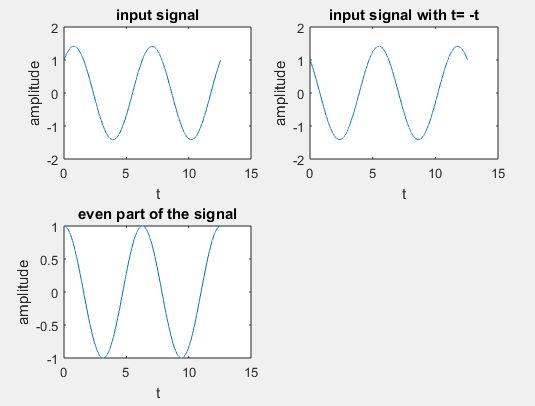
t=0:.001:4*pi;
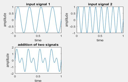
x=sin(t)+cos(t); % x(t)=sin(t)+cos(t)
subplot(2,2,1)
plot(t,x)
xlabel(‘t’);
ylabel(‘amplitude’)
title(‘input signal’)
y=sin(-t)+cos(-t); % y(t)=x(-t)
subplot(2,2,2)
plot(t,y)
xlabel(‘t’);
ylabel(‘amplitude’)
title(‘input signal with t= -t’)
even=(x+y)/2;
subplot(2,2,3)
plot(t,even)
xlabel(‘t’);
ylabel(‘amplitude’)
title(‘even part of the signal’)
Odd signal:
When a signal is distinguished as odd signal when it satisfies the below condition, for a continuous time signal x(t).
x(-t)=-x(t) for all t
When a signal is distinguished as odd signal when it satisfies the below condition, for a Discrete time signal x(n).
x(-n)=-x(n) for all n
Sine wave is an example of odd signal.
clc;
close all;
clear all;
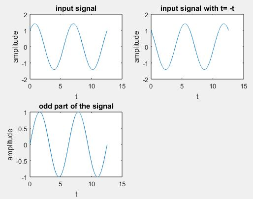
t=0:.001:4*pi;
x=sin(t)+cos(t); % x(t)=sint(t)+cos(t)
subplot(2,2,1)
plot(t,x)
xlabel(‘t’);
ylabel(‘amplitude’)
title(‘input signal’)
y=sin(-t)+cos(-t);
subplot(2,2,2)
plot(t,y)
xlabel(‘t’);
ylabel(‘amplitude’)
title(‘input signal with t= -t’)
odd=(x-y)/2;
subplot(2,2,3)
plot(t,odd)
xlabel(‘t’);
ylabel(‘amplitude’);
title(‘odd part of the signal’);
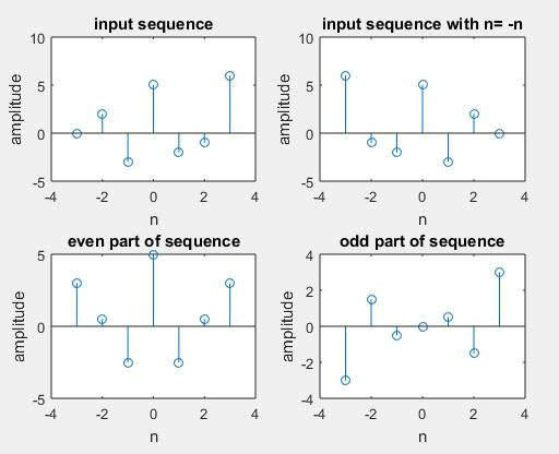
Even And Odd Parts Of Sequence:
clc;
close all;
clear all;
% Even and odd parts of a sequence
x1=[0,2,-3,5,-2,-1,6];
n=-3:3;
y1= fliplr(x1);%y1(n)=x1(-n)
figure;
subplot(2,2,1);
stem(n,x1);
xlabel(‘n’);
ylabel(‘amplitude’);
title(‘input sequence’);
subplot(2,2,2);
stem(n,y1);
xlabel(‘n’);
ylabel(‘amplitude’);
title(‘input sequence with n= -n’);
even1=.5*(x1+y1);
odd1=.5*(x1-y1);
% plotting even and odd parts of the sequence
subplot(2,2,3);
stem(n,even1);
xlabel(‘n’);
ylabel(‘amplitude’);
title(‘even part of sequence’);
subplot(2,2,4);
stem(n,odd1);
xlabel(‘n’);
ylabel(‘amplitude’);
title(‘odd part of sequence’);