Fourier Transform:
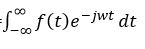
A mathematical way of converting a non-periodic function from amplitude v/s time domain to the amplitude v/s frequency domain. The Fourier transform as follows. If let’s consider ƒ is a function which is zero outside of some interval [−L/2, L/2]. If suppose the condition is T ≥ L we may expand ƒ in a Fourier series with the interval period [−T/2,T/2], where the “amount” of the wave e2πinx/T for the Fourier series it is given as ƒ definition Fourier Transform of signal f(t) is determined as
F(w)=
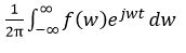
Let’s consider the inverse Fourier Transform of signal F(w) is determined as
F(t) =
Program:
clc;
clear all;
close all;
fs=1000;
N=1024; % length of fft sequence
t=[0:N-1]*(1/fs);
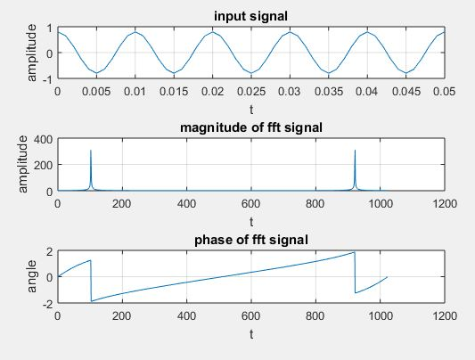
% input signal
x=0.8*cos(2*pi*100*t);
subplot(3,1,1);
plot(t,x);
axis([0 0.05 -1 1]);
grid;
xlabel(‘t’);
ylabel(‘amplitude’);
title(‘input signal’);
% Fourier transform of given signal
x1=fft(x);
% magnitude spectrum
k=0:N-1;
Xmag=abs(x1);
subplot(3,1,2);
plot(k,Xmag);
grid;
xlabel(‘t’);
ylabel(‘amplitude’);
title(‘magnitude of fft signal’)
%phase spectrum
Xphase=angle(x1);
subplot(3,1,3);
plot(k,Xphase);
grid;
xlabel(‘t’);
ylabel(‘angle’);
title(‘phase of fft signal’);
Bilateral Laplace transform:
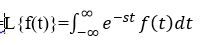
Let’s consider the Bilateral Laplace transforms: The Laplace transform for the given signal f(t) can be determined as follows:
F(s)=L{f(t)}=
If let’s consider the inverse Laplace transform is determined by the following formula:
F(t) =L-1{f(s)}=
Program:
clc;
clear all;
close all;
%representation of symbolic variables
syms f t w s;
%laplace transform of t
f=t;
z=laplace(f);
disp(‘the laplace transform of f = ‘);
disp(z);
% laplace transform of a signal
%f1=sin(w*t);
f1=-1.25+3.5*t*exp(-2*t)+1.25*exp(-2*t);
v=laplace(f1);
disp(‘the laplace transform of f1 = ‘);
disp(v);
lv=simplify(v);
pretty(lv)
%inverse laplace transform
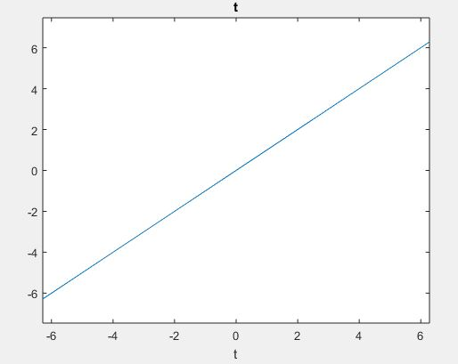
y1=ilaplace(z);
disp(‘the inverse laplace transform of z = ‘);
disp(y1);
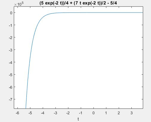
y2=ilaplace(v);
disp(‘the inverse laplace transform of v = ‘);
disp(y2);
ezplot(y1);
figure;
ezplot(y2)
output:
The Laplace transform of f = 1/s^2
The laplace transform of f1 = 5 \(4*(s + 2)) + 7/(2*(s + 2)^2) – 5/(4*s)
The inverse Laplace transform of z = t
The inverse Laplace transform of v =
(5*exp (-2*t))/4 + (7*t*exp(-2*t))/2 – 5/4