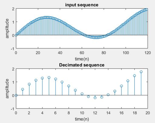
Decimation process implementation:
Theory:
“Decimation” is that the process of reducing the rate.
“Down sampling” may be a more specific term that refers to only the method of throwing away samples, without the low pass filtering operation. The most important reason to decimate is simply to reduce the sampling rate at the output of 1 system so a system operating at a lower rate can input the signal. But the away more common motivation for decimation is to scale back the value of processing: the calculation and the memory required to implement a DSP system generally is proportional to the rate, therefore the use of a lower rate usually leads to a cheaper implementation.
Steps involved in performing decimation process:
Step I: let’s define down sampling factor and input frequencies f1 and f2
Step II: And Represent input sequence with frequencies f1 and f2
Step III: To perform the decimation on input signal by using MatLab command decimate.
Step IV: Next plot the input and output sequence.
Program:
clc;
clear all;
close all;
D=input(‘enter the down sampling factor’);
L=input(‘enter the length of the input signal’);
f1=input(‘enter the frequency of first sinusoidal’);
f2=input(‘enter the frequency of second sinusoidal’);
n=0:L-1;
x=sin(2*pi*f1*n)+sin(2*pi*f2*n);
y=decimate(x,D,’fir’);
subplot(2,1,1);
stem(n,x(1:L));
title(‘input sequence’);
xlabel(‘time(n)’);
ylabel(‘amplitude’);
subplot(2,1,2)
m=0:(L/D)-1;
stem(m,y(1:L/D));
title(‘Decimated sequence’);
xlabel(‘time(n)’);
ylabel(‘amplitude’);
Output:
enter the down sampling factor6
enter the length of the input signal120
enter the frequency of first sinusodal0.002
enter the frequency of second sinusodal0.01

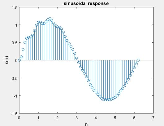
SINUSOIDAL SIGNAL GENERATION THROUGH FILTERING PROCESS:
One of the most important applications of an LTI discrete-time system is to pass certain frequency components in an input sequence with no distortion and block other frequency components. Such systems are called digital filters. The key to the filtering process is the inverse Discrete Fourier transform, which expresses an arbitrary input sequence as a the linear weighted sum of an infinite number of exponential sequences, or equivalently, as a the linear weighted sum of sinusoidal sequences. As a result, by appropriately choosing the values of magnitude function of the LTI digital filter at frequencies like the frequencies of the sinusoidal components of the input, a number of these sinusoidal sequences can be selectively heavily attenuated or filtered with reference to the others.
Program:
close all;
clear all;
clc;
b=[1];
a=[1,-1,0.9];
n=[-20:120];
t=0:0.1:2*pi;
x=sin(t);
s=filter(b,a,x);
stem(t,s);
title(‘sinusoidal response’);
xlabel(‘n’);
ylabel(‘s(n)’);

