Steps involved in performing FIR filter operation
Step I: Let’s enter the pass band frequency (fp) and stop band frequency (fq).
Step II: And then get the sampling frequency (fs), length of window (n).
Step III: Next calculate cut off frequency.
Step IV: Use the boxcar, hamming, Blackman Commands for designing window.
Step V: And then design filter by using above parameters.
Step VI: To find frequency response of the filter by using matlab command freqz.
Step VII: Then plot the magnitude response and phase response of the filter.
Program:
clc;
clear all;
close all;
n=20;
fp=300;
fq=200;
fs=1000;
fn=2*fp/fs;
window=blackman(n+1);
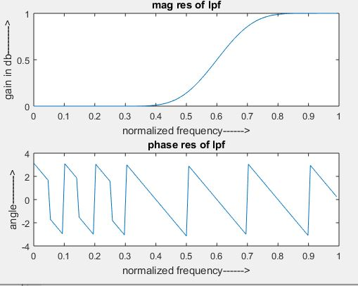
b=fir1(n,fn,’high’,window);
[H W]=freqz(b,1,128);
subplot(2,1,1);
plot(W/pi,abs(H));
title(‘mag res of lpf’);
ylabel(‘gain in db——–>’);
xlabel(‘normalized frequency——>’);
subplot(2,1,2);
plot(W/pi,angle(H));
title(‘phase res of lpf’);
ylabel(‘angle——–>’);
xlabel(‘normalized frequency——>’);
Steps involved in performing IIR filter operation
Step I: Now enter the pass band ripple (rp) and stop band ripple (rs).
Step II: while the pass band frequency (wp) and stop band frequency (ws).
Step III: Then Get the sampling frequency (fs).
Step IV: Then calculate the normalized pass band frequency, and normalized stop band frequency w1 and w2 respectively.
Step V : Make using the following function for calculating the Butterworth filter order [n,wn]=buttord(w1,w2,rp,rs ) and Chebyshev filter order [n,wn]=cheb1ord(w1,w2,rp,rs)
Step VI: Let’s design the nth order digital high pass Chebyshev or Butterworth filter using the following commands. Butterworth filter [b,a]=butter (n, wn,’high’) Chebyshev filter [b,a]=cheby1 (n, 0.5, wn,’high’)
Step VII: In order to find the digital frequency response of the filter by using ‘freqz ( )’ function
Step VIII: Then calculate the magnitude for the frequency response in decibels (dB) mag=20*log10 (abs (H))
Step IX: Then plot the magnitude response [magnitude in dB Vs normalized frequency]
Step X: Next calculate the phase response using angle (H).
Step XI: Then plot the phase response [phase in radians Vs normalized frequency (Hz)].
Program:
clc;
clear all;
close all;
disp(‘enter the IIR filter design specifications’);
rp=input(‘enter the passband ripple’);
rs=input(‘enter the stopband ripple’);
wp=input(‘enter the passband freq’);
ws=input(‘enter the stopband freq’);
fs=input(‘enter the sampling freq’);
w1=2*wp/fs;w2=2*ws/fs;
[n,wn]=buttord(w1,w2,rp,rs,’s’);
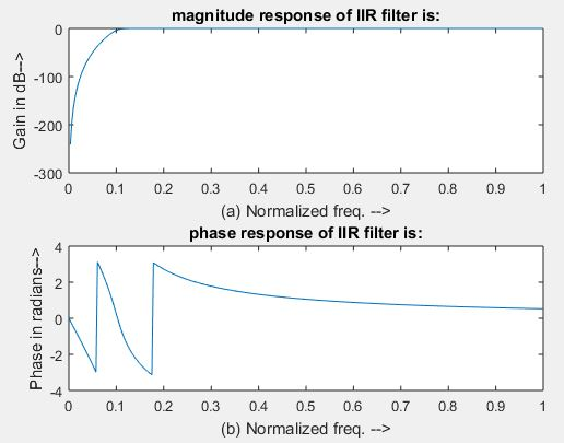
disp(‘Frequency response of IIR HPF is:’);
[b,a]=butter(n,wn,’high’,’s’);
w=0:.01:pi;
[h,om]=freqs(b,a,w);
m=20*log10(abs(h));
an=angle(h);
figure, subplot(2,1,1);plot(om/pi,m);
title(‘magnitude response of IIR filter is:’);
xlabel(‘(a) Normalized freq. –>’);
ylabel(‘Gain in dB–>’);
subplot(2,1,2);plot(om/pi,an);
title(‘phase response of IIR filter is:’);
xlabel(‘(b) Normalized freq. –>’);
ylabel(‘Phase in radians–>’);