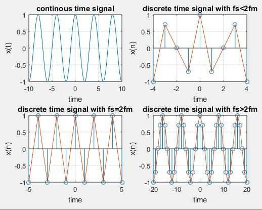
Sampling theorem:
Sampling theorem is used to convert analog signal into discrete time signal.it has applications in digital signal processing and digital communication. Sampling theorem is determined has that if the sampling rate in any pulse modulation system exceeds twice the maximum frequency of the message signal, with this the receiver will reconstructed the signal with minimum distortion.
Whereas,
fs is the sampling rate
fm is the maximum frequency of message signal
Then sampling theorem can be expressed in mathematical form as
Fs≥ 2fm
Well 2fm is determined as Nyquist rate.
It the condition is
Fs≤2fm
It is defined as aliasing effect it occurred when the sampling rate is less than twice the maximum frequency of the message signal.
Fs=sampling rate
Program:
clc;
clear all;
close all;
t=-10:.01:10;
T=4;
fm=1/T;
x=cos(2*pi*fm*t);
subplot(2,2,1);
plot(t,x);
xlabel(‘time’);
ylabel(‘x(t)’);
title(‘continous time signal’);
grid;
n1=-4:1:4;
fs1=1.6*fm;
fs2=2*fm;
fs3=8*fm;
x1=cos(2*pi*fm/fs1*n1);
subplot(2,2,2);
stem(n1,x1);
xlabel(‘time’);
ylabel(‘x(n)’);
title(‘discrete time signal with fs<2fm’);
hold on;
subplot(2,2,2);
plot(n1,x1);
grid;
n2=-5:1:5;
x2=cos(2*pi*fm/fs2*n2);
subplot(2,2,3);
stem(n2,x2);
xlabel(‘time’);
ylabel(‘x(n)’);
title(‘discrete time signal with fs=2fm’);
hold on;
subplot(2,2,3);
plot(n2,x2)
grid;
n3=-20:1:20;
x3=cos(2*pi*fm/fs3*n3);
subplot(2,2,4);
stem(n3,x3);
xlabel(‘time’);
ylabel(‘x(n)’);
title(‘discrete time signal with fs>2fm’)
hold on;
subplot(2,2,4);
plot(n3,x3)
grid;
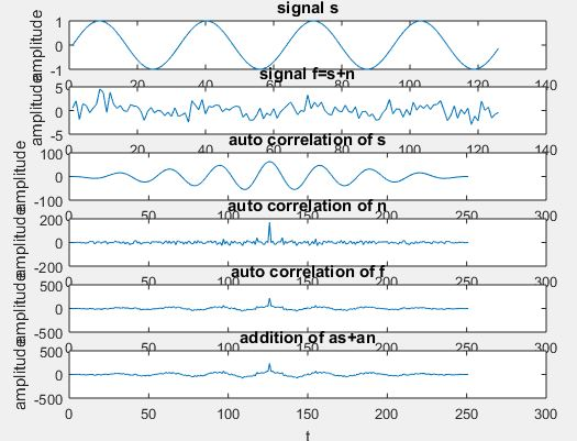
Noise removal by using cross-correlation/autocorrelation
Detection of the periodic signal conceal by random noise is of great importance .The noise signal encountered in practice may be a signal with random amplitude variations. A signal is uncorrelated with any periodic signal. If s(t) is a periodic signal and n(t) is a noise signal then.
clc;
clear all;
close all;
t=0:0.2:pi*8;
%input signal
s=sin(t);
subplot(6,1,1);
plot(s);
title(‘signal s’);
xlabel(‘t’);
ylabel(‘amplitude’);
%generating noise
n = randn([1 126]);
%noisy signal
f=s+n;
subplot(6,1,2)
plot(f);
title(‘signal f=s+n’);
xlabel(‘t’);
ylabel(‘amplitude’);
%autocorrelation of input signal
as=xcorr(s,s);
subplot(6,1,3);
plot(as);
title(‘auto correlation of s’);
xlabel(‘t’);
ylabel(‘amplitude’);
%autocorrelation of noise signal
an=xcorr(n,n);
subplot(6,1,4)
plot(an);
title(‘auto correlation of n’);
xlabel(‘t’);
ylabel(‘amplitude’);
%autocorrelation of transmitted signal
cff=xcorr(f,f);
subplot(6,1,5)
plot(cff);
title(‘auto correlation of f’);
xlabel(‘t’);
ylabel(‘amplitude’);
%autocorrelation of received signal
hh=as+an;
subplot(6,1,6)
plot(hh);
title(‘addition of as+an’);
xlabel(‘t’);
ylabel(‘amplitude’);