Thursday, March 5, 2026
Home Blog Page 10

Tree , Graph searching for problem solving as state space, Formalizing search in a graph,

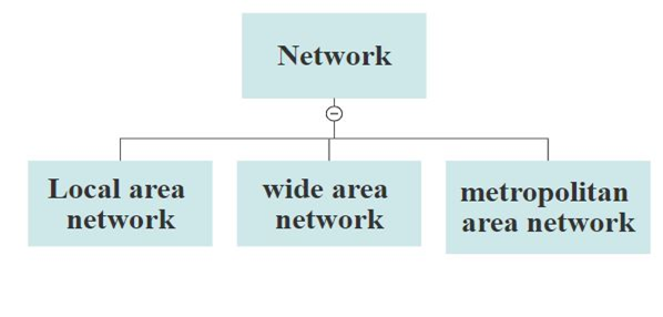
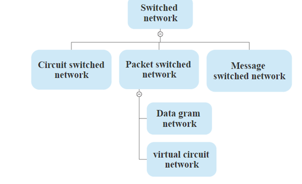
•   A tree is graph connected  without any cycles.

•  Trees comes with different types: tournament brackets, family trees, organizational charts and decision trees. In the above figure  there is a path between a to b and b to a this forms  a cycle. Here in tree no such  cycles are formed.


Graph searching for problem solving as state space

•  Graph searching for problem solving as state space  search  is to find a sequence of actions to achieve a goal as searching for paths in a directed graph.

•  To solve the problem ,We define the underlying search space  and then apply a search algorithm.

•  Searching  in  graphs, therefore, provides  an appropriate  abstract model of problem solving , independent of the particular domain.

Formalizing search in a graph

  1. To formalize search in a graph, first we need to define a state space. Lets a say the state space is a graph    of vertices and edges  i.e., (V,E)

• V is a set of nodes and

•  E is a set of arcs , directed from a node to another node.

2. Each node  refers to a simple node  data structure that contains a state description  and other information  such as the parent of the node , operator that generated the node from that parent, and other book keeping data.

3. Each arc corresponds to an instance of one of the operators.

4.Whenever we are formalizing search in state space  , we are converting the entire state space into nodes with each operator with some instances that takes me  to next nodes which ends up in a directed graph. This searching in a directed graph for a path from Start to Goal gives the solution.

5. Each arc in a directed graph has a fixed positive cost associated with it corresponding to the cost of the operator.

6. Each node has a set of successor nodes corresponding to all of the legal operators as that can be applied to the source node state.

•   expanding a node means  it is a continuous process of generating  all the successor nodes and add them to their associated arcs.

7.  One or more nodes are designated as the start node later there will be a  goal test predicate that  is applied to a state to determine if its associated node is goal node.

8. A solution is a sequence of operators that is associated with a path in a state space from a start node to goal node.

Notion of path in a graph

The notion of a path in a graph is  clear and is shown below

•             Suppose G (V,E) is a graph with vertices v¬0, v1,v2,……,vk. and edges are e1,e2,……..,ek in which edge  ei={vi-1,vi} for i= 1,…,k.

•             The alternating sequence that I get of vertices and edges , starting from the vertice v0 to vk is a path from  v0 to vk of length k. The length is the number of edges and it is not the number of vertices.

•             The length of the path is 1,2, 3 and 4 so here is a 4 length path. And the path is made up of edges e1,e2,e3,e4 and it had vertices va,  vb,  vc  .So the path from the start to goal for the given graph is  s, e1,va, e2,vb,e3,vc,e4, g.

 Directed graph(Digraph)

A directed graph  or a Digraph in short consists of  a set V of vertices and asset E of directed edges.

•A directed edge is an ordered pair of elements of V .put another  way the pair  G(V,E) with E is a sub set of VxV is a digraph

•Digraphs allow for loops of the form (a, a), it is also possible to have two edges (a, b) and (b, a)  between the vertices  a and b

•We take the ordering of pairs in E to give each edge a direction: namely the edge (a, b) goes from a to b.

•If we draw a digraph ,we draw the edge (a, b) as an arrow from a to b.

Example:

V= {a, b, c, d}

E= {(a ,b),(a, c),(b, a),(c, c),(d, c)}

UNINFORMED SEARCH

Uninformed search does not have any domain knowledge. Here we are going to learn about some uniformed search strategies. Before getting into this take a review on problem solving as search, state spaces, graph searching and generic searching algorithms.

We have previously learnt about the general definitions of problem solving as search and state space

In general ,problem solving as a state space can be defined as mathematical form of finding a path from start node to a goal node in the directed path.

Graph:

A graph,  G  has  two sets , set  V of vertices and a set E of edges. Vertex set is the collection of letters or numbers.

•  The set of edges consists of  doubleton subsets of V. That is E is the subset of {a, b} such that a, b belongs to V  and a≠ b.

•  We denote the graph by G(V,E).

        If G (V,E) is a graph and {a, b} belongs to E ; Then we say vertices a and b are adjacent and the edge {a, b} Joins them or connects them or is incident on them .We call a and b the endpoints of the edge .

•   Two edges such as {a, b} and { b, c} shares same vertex  with a≠ c, are adjacent to each other.

Network categories

Network categories:

Depending upon the size of the network, distance, and physical characteristics network is categorized into three types local area network(LAN), wide area network (WAN), and metropolitan area network(MAN).

Fig: Categories Of Networks

Local area network(LAN):

Local area network size is limited to few kilometers, which is mainly depends on privately-owned organizations. Based upon the requirements of the organization different types of technologies are used, LAN is very simple which will connect two personal computers within the same building, office, and home.

LAN can share some resources between two PC’s or workstations, these resources sharing may include hardware or software, or information. Let us consider some examples of LAN which may found in some engineering workstations or accounting Personal computers. One of them found in business environments, like linking a workgroup of task-related computers. The large capacity disk drive is considered as a server to clients, while the size of LAN may depend on licensing restrictions and the number of users per copy of the software. Its speed is 100 or 1000 Mbps. The most commonly used LAN topologies are ring, star, and bus.

Wide Area Network(WAN):

For transferring video, images, data, and audio information even for long-distance or across the country or all over the world we require a large network that may be a wide area network which will act as a backbone to connect the internet or simple dial-up line that connect a home computer to the internet. There are two types of WAN which are switched WAN and point to point WAN from this the switched WAN is connected to the end systems, which is usually considered as a router it will connect to another WAN or LAN. Point to point WAN is normally a line leased from a telephone or cable TV provider which is connected to a home computer or a small LAN to an internet service provider(ISP).

Let’s consider examples for both switched and point to point WAN, asynchronous transfer mode(ATM) network is an example of switched WAN it has fixed-size data packets called cells.

Metropolitan Area Network(MAN):

The size of the MAN network is in between LAN and WAN, which will cover the distance area inside a city or town. The best example of a MAN network is the part of the telephone company network that provides a high-speed DSL line to the customer.

Gibbs Phenomenon and Verifying its stability for the given Unit step, unit sample, and sinusoidal response of the LTI system

0

Verifying its stability for the given Unit step, unit sample, and sinusoidal response of the LTI system

Verifying its stability for the given Unit step, unit sample, and sinusoidal response of the LTI system. A discrete-time system performs an operation on an input supported predefined criteria to supply a modified output. The input x(n) is that the system excitation and y(n) is that the system response. If the input of the system is unit impulse i.e. x(n) = δ(n) then the output of the system is understood as impulse response denoted by h(n)where h(n)= T[δ(n)] we all know that any arbitrary sequence x(n) can be represented as a weighted sum of discrete impulses.

Program:

%given difference equation y(n)-y(n-1)+.9y(n-2)=x(n);

clc;

clear all;

close all;

b=[1];

a=[1,-1,.9];

n =0:3:100;

%generating impulse signal

x1=(n==0);

%impulse response

y1=filter(b,a,x1);

subplot(3,1,1);

stem(n,y1);

xlabel(‘n’);

ylabel(‘y1(n)’);

title(‘impulse response’);

%generating step signal

x2=(n>0);

% step response

y2=filter(b,a,x2);

subplot(3,1,2);

stem(n,y2);

xlabel(‘n’);

ylabel(‘y2(n)’)

title(‘step response’);

%generating sinusoidal signal

t=0:0.1:2*pi;

x3=sin(t);

% sinusoidal response

y3=filter(b,a,x3);

subplot(3,1,3);

stem(t,y3);

xlabel(‘n’);

ylabel(‘y3(n)’);

title(‘sin response’);

% verifying stability

figure;

zplane(b,a);

Gibbs Phenomenon

The Gibbs phenomenon, the Fourier series of a piecewise continuously differentiable periodic function behaves at a jump discontinuity. The n the approximated function shows amounts of ripples at the points of discontinuity. This is known as the Gibbs Phenomena. Partial sum of the Fourier series has large oscillations near the jump, which could increase the utmost of the partial sum above that of the function itself. The overshoot doesn’t die out because the frequency increases, but approaches a finite limit The Gibbs phenomenon involves both the very fact that Fourier sums overshoot at a jump discontinuity, and that this overshoot does not die out as the frequency increases.

Program:

% Gibb’s phenomenon.

clc;

clear all;

close all;

t=linspace(-2,2,2000);

u=linspace(-2,2,2000);

sq=[zeros(1,500),2*ones(1,1000),zeros(1,500)];

k=2;

N=[1,3,7,19,49,70];

for n=1:6;

an=[];

for m=1:N(n)

 an=[an,2*k*sin(m*pi/2)/(m*pi)];

end;

fN=k/2;

for m=1:N(n)

 fN=fN+an(m)*cos(m*pi*t/2);

end;

nq=int2str(N(n));

subplot(3,2,n),plot(u,sq,’r’);hold on;

plot(t,fN); hold off; axis([-2 2 -0.5 2.5]);grid;

xlabel(‘Time’), ylabel(‘y_N(t)’);title([‘N= ‘,nq]);

end;

VERIFICATION OF BOTH LINEAR AND TIME INVARIANT SYSTEMS

0

LINEARITY PROPERTY:

If any system is claimed to be linear if it satisfies the superposition principal. Superposition principal state that Response to a weighted sum of input adequate to the corresponding weighted sum of the outputs of the system to every of the individual input signals.
If x(n) may be a input and y(n) may be a output then

y(n)=T[x(n)]

 y1(n) =T[x1(n)] and y2(n)=T[x2(n)]

 x3 =[a*x1(n) +b *x2(n) ]

Y3(n) = T [x3(n)]

 T [a*x1(n) + b*x2(n)] = a y1(n) +  b y2(n)

Program:

clc;

close all;

clear all;

% Verification of Linearity of a given System.

% a) y(n)=nx(n) b) y=x^2(n)

n=0:40;

a1=input(‘enter the scaling factor a1=’);

a2=input(‘enter the scaling factor a2=’);

x1=cos(2*pi*0.1*n);

x2=cos(2*pi*0.4*n);

x3=a1*x1+a2*x2;

%y(n)=n.x(n);

y1=n.*x1;

y2=n.*x2;

y3=n.*x3;

yt=a1*y1+a2*y2;

yt=round(yt);

y3=round(y3);

if y3==yt

 disp(‘given system [y(n)=n.x(n)]is Linear’);

else

 disp(‘given system [y(n)=n.x(n)]is non Linear’);

end

%y(n)=x(n).^2

x1=[1 2 3 4 5];

x2=[1 4 7 6 4];

x3=a1*x1+a2*x2;

y1=x1.^2;

y2=x2.^2;

y3=x3.^2;

yt=a1*y1+a2*y2;

if y3==yt

 disp(‘given system [y(n)=x(n).^2 ]is Linear’);

else

 disp(‘given system is [y(n)=x(n).^2 ]non Linear’);

end

Output will obtained as

Enter the scaling factor a1=3

Enter the scaling factor a2=5

Given system [y(n) =n.x(n)]is Linear

Given system is [y(n) =x(n).^2 ]non Linear

Time-Invariant System:

A system is named time-invariant if its input-output characteristics don’t change with time. X(t) is the input and Y(t) will be the output, X(t-k) is a delayed form of input by k seconds, Y(t-k) is delayed form of output by k seconds.

 If Y(t)=T[X(t)] while Y(t-k)=T[X(t-k)] then system is time invariant system.

clc;

close all;

clear all;

% Verification of your Time Invariance of a Discrete System

% a)y=x^2(n) b) y(n)=nx(n)

clc;

clear all;

close all;

n=1:9;

x(n)=[2 1 4 3 6 5 8 7 9];

d=3; % some time delay

xd=[zeros(1,d),x(n)];%x(n-k)

y(n)=x(n).^2;

yd=[zeros(1,d),y];%y(n-k)

disp(‘transformation of delay signal yd:’);

disp(yd)

dy=xd.^2; % T[x(n-k)]

disp(‘delay of transformation signal dy:’);

disp(dy)

if dy==yd

 disp(‘given system [y(n)=x(n).^2 ]is time invariant’);

else

 disp(‘given system is [y(n)=x(n).^2 ]not time invariant’);

end

y=n.*x;

yd=[zeros(1,d),y(n)];

disp(‘transformation of delay signal yd:’);disp(yd);

n1=1:length(xd);

dy=n1.*xd;

disp(‘delay of transformation signal dy:’);disp(dy);

if yd==dy

 disp(‘given system [y(n)=nx(n)]is a time invariant’);

else

 disp(‘given system [y(n)=nx(n)]not a time invariant’);

 end

Output:

Transformation of delay signal yd:

     0     0     0     4     1    16     9    36    25    64    49    81

Delay of transformation signal dy:

     0     0     0     4     1    16     9    36    25    64    49    81

Given system [y(n)=x(n).^2 ]is time invariant

Transformation of delay signal yd:

     0     0     0     2     2    12    12    30    30    56    56    81

Delay of transformation signal dy:

     0     0     0     8     5    24    21    48    45    80    77   108

Given system [y(n)=nx(n)]not a time invariant

Types of Switching Techniques In Networking

Switching Techniques Types In Networking:

A switch is hardware are software equipment that is used to provide the connection between two or more than two devices. And a switched network is made of many interlinked nodes.

                    Fig: Types of the switched network 

Circuit Switching:

Circuit switching similarly looks like a telephone call, in which it establishes a dedicated physical path between sender and receiver in order to transmit information, this path is continued until total data is sent to the receiver. This path is not shared with others until the sender and receiver stop communication.
Let us consider an example of circuit switching when you set up a call with someone over the phone, a dedicated path is established between your phone and another person’s phone through a switch this path will continue until the call ends.
It mainly used for telephone communication, and computer to computer communication in circuit switching is not so much efficient.

Advantages:
Circuit switching is very simple.
Delay at every node is negligible.
Disadvantages:
Circuit switching is less flexible.
In this channel, capacity is not properly utilized.
It is used for voice communication and does not use for data communication.


Packet switching:

While considering the disadvantages of circuit switching, packet switching is developed. In which switching technology to provide communication between two computers.When compared with circuit switching packet switching as no dedicated path for data transmission between sender and receiver. In this, all the packets that belong to the same message do not need to go in the same route to reach the destination. Packets go through a different route to reach the destination.
In this packet switching type, the data is transmitted in the form of small discrete blocks called packets. Once the best path is selected between source and destination then the sender will send to data, it converts them into packets and routes them to destination.
The packet routing is decided by network-layer protocols. Further packet switching can be classified into two types.
Datagram Approach:
In this datagram packet switching type, each packet is sent from the source to the destination through different routes.
Virtual Approach:
In this virtual circuit, all packets belonging to the same message are sent the same route from source to destination.
Message switching:
Message switching is best known as the store and forward approach for an entire message. In this method a computer receives a message, stores it until the appropriate route is free then sends it along that route.

Goal of decomposable production system


The main goal of Decomposable Production System is to replace a problem goal by set of sub goals .If the sub goals are solved then the main goal is also solved

Explaining problems in terms of decomposable production system allows us to be indefinite about whether we are decomposing problem goals or problem states.


Knowledge of the problem domain:


For efficient working of AI systems, good problem knowledge is required. This knowledge can be subdivided into three categories.

  1. Declarative Knowledge
  2. Procedural Knowledge
  3. Control Knowledge
    Declarative Knowledge
    Declarative knowledge is knowledge about a problem that is represented in the global database. Declarative knowledge includes specific facts.
    Procedural Knowledge
    Procedural Knowledge is Knowledge about a problem that is represented in rules; general information that allows us to manipulate the declarative knowledge.
    Control Knowledge
    Control knowledge is the knowledge about different processes, structures and Strategies used for coordinating the entire problem solving process.

AND-OR Graph

Nodes labeled by component databases have sets of successor nodes each labeled by one of the components. These nodes are called AND nodes because in order to process the compound database to termination all of the component database must be processed to termination.  In the above figure 2,  this node here in order to process C B Z to termination, C,B and Z needs to be processed to termination. In order  to process BM to termination both B and M needs to be processed to termination; so  on and so forth. This type of termination which requires all the successors of single label to terminate for processing that single label is known as AND node.  Another important thing that one needs to realize is that the successor nodes are labeled by the result of rule application.

  Here in the next step in order to process C, we have either of two ways that is we can terminate C by terminating DL or we can terminate with  BM.  Here we can follow any of the successor not both. They are referred to as the ‘OR’ nodes. Because , in order to process a component database to termination , the database resulting from only either DL or BM must be processed to termination. These are referred to as ‘or’ nodes.

 The structure called AND-OR graphs  are useful for depicting the activity of production systems. So the decomposable production system if you see above has these nodes that is  AND  and OR are important because if a component database is AND  then all of the component databases need to be moved to termination. So, that is the AND node here …examples  of AND nodes in the above figure are

  1. C B Z : C, B ,Z  (To process C B Z  all the three successors C,B,Z needs to be terminated)
  2. Z: B,M,B (To process Z all the three successors B, M, B needs to be terminated)

 The above are the AND nodes, here all of them needs to be moved to the termination.

On the other hand , we also have  OR nodes  in the above figure .For example, In order to process the C we can terminate any of the successors (i.e., D,L or B,M).

So, finally we can say that the notion of decomposable production system encompass a technique often called problem Reduction in AI. We have reduced the problem of taking C B Z to termination. To the problem of taking C, B and Z individually to termination.

correlation between two signals and sequences

0

CORRELATION:

The concept correlation can be defined as similarities of two waveforms. It may determine if signal x1(t) waveform contain an amount c2x2(t) of that particular waveform x2(t) in the interval of (t1, t2). It is a measure of the degree to which two sequences are similar.Correlation is of two types cross correlation and autocorrelation.

Cross correlation:

Cross-correlation between two signals indicates what proportion one signal is said to the time-delayed version of another signal.

clc;

close all;

clear all;

% two input sequences

x=input(‘enter input sequence’);

h=input(‘enter the impulse sequence’);

subplot(2,2,1);

stem(x);

xlabel(‘n’);

ylabel(‘x(n)’);

title(‘input sequence’);

subplot(2,2,2);

stem(h);

xlabel(‘n’);

ylabel(‘h(n)’);

title(‘impulse sequence’);

% cross correlation between two sequences

y=xcorr(x,h);

subplot(2,2,3);

stem(y);

xlabel(‘n’);

ylabel(‘y(n)’);

title(‘ cross correlation between two sequences ‘);

Autocorrelation:

The auto correlation function is a special form of cross correlation function.

clc;

close all;

clear all;

% two input sequences

x=input(‘enter input sequence’);

h=input(‘enter the impulse sequence’);

subplot(2,2,1);

stem(x);

xlabel(‘n’);

ylabel(‘x(n)’);

title(‘input sequence’);

subplot(2,2,2);

stem(h);

xlabel(‘n’);

ylabel(‘h(n)’);

title(‘impulse sequence’);

% auto correlation of input sequence

z=xcorr(x,x);

subplot(2,2,4);

stem(z);

xlabel(‘n’);

ylabel(‘z(n)’);

title(‘auto correlation of input sequence’);

crosscorrelation between two signals

clc;

close all;

clear all;

% cross correlation between two signals

% generating two input signals

t=0:0.2:10;

x1=3*exp(-2*t);

h1=exp(t);

figure;

subplot(2,2,1);

plot(t,x1);

xlabel(‘t’);

ylabel(‘x1(t)’);

title(‘input signal’);

subplot(2,2,2);

plot(t,h1);

xlabel(‘t’);

ylabel(‘h1(t)’);

title(‘impulse signal’);

% cross correlation

subplot(2,2,3);

z1=xcorr(x1,h1);

plot(z1);

xlabel(‘t’);

ylabel(‘z1(t)’);

title(‘cross correlation ‘);

% auto correlation

subplot(2,2,4);

z2=xcorr(x1,x1);

plot(z2);

xlabel(‘t’);

ylabel(‘z2(t)’);

title(‘auto correlation ‘);