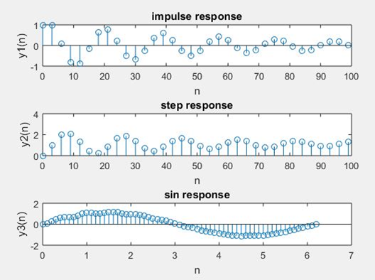
Verifying its stability for the given Unit step, unit sample, and sinusoidal response of the LTI system
Verifying its stability for the given Unit step, unit sample, and sinusoidal response of the LTI system. A discrete-time system performs an operation on an input supported predefined criteria to supply a modified output. The input x(n) is that the system excitation and y(n) is that the system response. If the input of the system is unit impulse i.e. x(n) = δ(n) then the output of the system is understood as impulse response denoted by h(n)where h(n)= T[δ(n)] we all know that any arbitrary sequence x(n) can be represented as a weighted sum of discrete impulses.
Program:
%given difference equation y(n)-y(n-1)+.9y(n-2)=x(n);
clc;
clear all;
close all;
b=[1];
a=[1,-1,.9];
n =0:3:100;
%generating impulse signal
x1=(n==0);
%impulse response
y1=filter(b,a,x1);
subplot(3,1,1);
stem(n,y1);
xlabel(‘n’);
ylabel(‘y1(n)’);
title(‘impulse response’);
%generating step signal
x2=(n>0);
% step response
y2=filter(b,a,x2);
subplot(3,1,2);
stem(n,y2);
xlabel(‘n’);
ylabel(‘y2(n)’)
title(‘step response’);
%generating sinusoidal signal
t=0:0.1:2*pi;
x3=sin(t);
% sinusoidal response
y3=filter(b,a,x3);
subplot(3,1,3);
stem(t,y3);
xlabel(‘n’);
ylabel(‘y3(n)’);
title(‘sin response’);
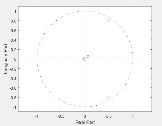
% verifying stability
figure;
zplane(b,a);
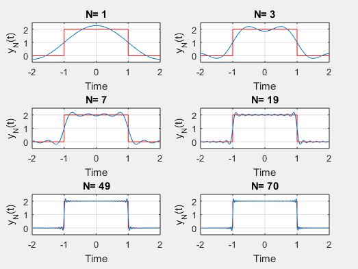
Gibbs Phenomenon
The Gibbs phenomenon, the Fourier series of a piecewise continuously differentiable periodic function behaves at a jump discontinuity. The n the approximated function shows amounts of ripples at the points of discontinuity. This is known as the Gibbs Phenomena. Partial sum of the Fourier series has large oscillations near the jump, which could increase the utmost of the partial sum above that of the function itself. The overshoot doesn’t die out because the frequency increases, but approaches a finite limit The Gibbs phenomenon involves both the very fact that Fourier sums overshoot at a jump discontinuity, and that this overshoot does not die out as the frequency increases.
Program:
% Gibb’s phenomenon.
clc;
clear all;
close all;
t=linspace(-2,2,2000);
u=linspace(-2,2,2000);
sq=[zeros(1,500),2*ones(1,1000),zeros(1,500)];
k=2;
N=[1,3,7,19,49,70];
for n=1:6;
an=[];
for m=1:N(n)
an=[an,2*k*sin(m*pi/2)/(m*pi)];
end;
fN=k/2;
for m=1:N(n)
fN=fN+an(m)*cos(m*pi*t/2);
end;
nq=int2str(N(n));
subplot(3,2,n),plot(u,sq,’r’);hold on;
plot(t,fN); hold off; axis([-2 2 -0.5 2.5]);grid;
xlabel(‘Time’), ylabel(‘y_N(t)’);title([‘N= ‘,nq]);
end;