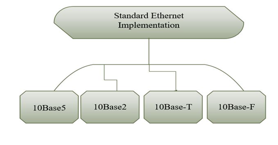
Saturday, May 2, 2026
Home Blog Page 9

TYPES OF ETHERNET

FAST ETHERNET:

In order to compete with LAN protocols fast ethernet was designed.it can transmit data 10 times faster when compared with standard ethernet. It has 100mbps data rate, which has same minimum and maximum frame length when compared with standard ethernet. A new feature which added to fast ethernet is auto negotiation, which was designed particularly for the following uses.

It allows a device of 10 mbps is connected to a device of 100mbps capacity.

It allow one device to have multiple capabilities.

It also allowed to check the hub’s capabilities.

Fast ethernet was implemented at physical layer which is categorized has follows two-wire or four-wire. In two-wire implementation further categorized into 5 UTP (100Base-TX) or fiber-optic cable (100Base-Fx). And four-wire is implemented for 3 UTP (100 BaseT4).

The encoding scheme used for fast ethernet:

Manchester encoding scheme required 200-M baud bandwidth for the data rate of 100Mbps, which seems unsuitable for medium such as twisted-pair. For this reason, the fast ethernet was designed with an alternative encoding/decoding scheme.

100Base-TX:

It uses two pair of twisted-pair cable i.e., 5 UTP or STP. In order to obtain good performance and bandwidth MLT-3 scheme was implemented. Where MLT-3 scheme is not a self-synchronous line-coding scheme, for this we are providing 4B/5B block coding to provide bit synchronization by preventing the occurrence of a long sequence of 0s and 1s. Which will improves the data rate of 125 Mbps.

100Base-FX:

It uses two pair of twisted-pair of fiber-optic cables. This will handle high bandwidth requirement by using simple encoding schemes. In order to provide the above requirement designer provided NRZ-I encoding scheme which has a bit synchronization problem for long sequence of 0s.to over the above problem designer used 4B/5B encoding scheme which can improves the data rates from 100 to 125 mbps, which can be easily handled by fiber-optics.

 100Base-T4: It was designed by using 3 or higher UTP. This implementation will be done by using four-pair of UTP for transmitting 100mbps. In this encoding/decoding schemes are more complicated, for this reason, the designer used three pairs of UTP category 3, however, can handle only 75 M baud each. In order to convert 100 Mbps to  75 M baud designer used 8B/6T  to satisfies the above requirement.

To plot autocorrelation and frequency response of a system in differential equation form for the given sequences

0

Theory for autocorrelation:

Auto Correlation Function Autocorrelation function is a measure of similarity between a signal & its time-delayed version. It is represented with R(k). While the autocorrelation function of x(n) is determined by

R11 (k) =R(k)=

Steps to perform auto correlation:

  • And the given input sequence is x[n].
  • Let the given impulse response of sequence h (n).
  • In order to auto correlation by using the matlab command xcorr.
  • Let’s plot the sequence x[n], h[n], z[n].
  • Next step is to display the result.

Program:

clc;

close all;

clear all;

% Let’s the two input sequences

x=input(‘enter input sequence’)

subplot(1,2,1);

stem(x);

xlabel(‘n’);

ylabel(‘x(n)’);

title(‘input sequence’);

% And the auto correlation of the given input sequence

z=xcorr(x, x);

disp(‘The values of z are = ‘);

disp(z);

subplot(1,2,2);

stem(z);

xlabel(‘n’);

ylabel(‘z(n)’);

title(‘auto correlation of input sequence’);

OUTPUT:

Enter input sequence [2 4 5 6]

x = 2     4     5     6

And the values of z are =

   12.0000   34.0000   58.0000   81.0000   58.0000   34.0000   12.0000

The frequency response of the signal in differential equation form:

Systems respond differently to inputs of different frequencies. Where some of the systems may amplify components with certain frequencies, and attenuate components of other frequencies. And the way system output is related to the system input with different frequencies is called the frequency response of the system. We can convert it to polar notation in the complex plane. This will provides us the magnitude and an angle. We call the angle the phase.

Amplitude Response: For each frequency, the magnitude represents the system’s tendency to amplify or attenuate the input signal.

Phase Response: The phase represents the system’s tendency to modify the phase of the input sinusoids.

Steps for obtaining frequency response of the signal:

  • And the given numerator coefficients of the given transfer function or difference equation.
  • And the given denominator coefficients of the given transfer function or difference equation
  • Let’s pass these coefficients to matlab command freqz to find frequency response.
  • In order to find magnitude and phase response by using matlab commands abs and angle.
  • Let’s plot the magnitude and phase response.

Program:

clc;

clear all;

b=input(‘Enter the numerator coefficients:’);

a=input(‘Enter the denominator coefficients:’);

[h,w]=freqz(b,a);

subplot(2,1,1);

plot(w/pi,abs(h));

grid;

xlabel(‘Normalised Frequency’);

ylabel(‘Magnitude in dB’);

title(‘Magnitude Response’);

subplot(2,1,2);

plot(w/pi,angle(h));

grid;

xlabel(‘Normalized Frequency’);

ylabel(‘phase in radians’);

title(‘Phase Response’);

CATEGORIES OF ETHERNET

DIFFERENT TYPES OF ETHERNET:

Depending on the encoding and decoding operation Ethernet are categorized into four:

STANDARD ETHERNET:

Standard Ethernet is implemented using digital signaling with the data rates of 10 Mbps.  Whereas at the sender, the data is converted into a digital signal using Manchester scheme. While at the receiver it uses Manchester scheme in order to decode the received signal. Manchester scheme is self-synchronous used for providing a transition at each bit interval. Standard Ethernet are categorized in to four types. They are as shown in below figure.

10BASE5 🙁 THICK ETHERNET)

This is the first implementation of standard Ethernet it is also known as thick ethernet. Name is derived based on the size of the cable. It is the first implementation which used bus topology with an external transceiver connected via a tap to a thick coaxial cable. Where transceiver is used for transmitting and receiving and detecting collisions. In order to provide separate path for transmitting and receiving data via transceiver cable. The maximum length of the cable should not exceed 500m, otherwise there will be degradation of the signal.

                 Transceiver          Thick coaxial cable maximum 500 m

10BASE 2: (THIN ETHERNET)

Thin ethernet is the second implementation of standard ethernet it also uses the bus topology, but the cable very thinner and more flexible. In this, the transceiver is the part of the network interface card (NIC), which is installed inside the station. It is very less expensive when compared with the thick ethernet, Its installation is simpler because of flexible. And the length of the thin ethernet is 185m.

10BASE-T: (TWISTED PAIR)

Twisted pair ethernet is the third implementation of the standard ethernet, which uses star topology. In which stations are connected to a hub via two pair of twisted cable. In this two pair of twisted cable create two paths between the station and hub. The maximum length of the cable is 100m.

10BASE-F: (FIBER CABLE)

10BASE-F uses a star topology to connect stations to a hub, the stations are connected to the hub using two fiber-optics cables.

TO PLOT LINEAR CONVOLUTION FOR THE GIVEN FINITE SEQUENCE

0

linear Convolution Theory:

Convolution is a mathematical way of combining the two signals to form a third signal. It is the only most vital technique in Digital Signal Processing. Using the strategy of impulse decomposition, systems are described by a sign called the impulse response. Convolution is vital because it relates the three signals of interest: the input, the output, and therefore the impulse response. When convolution is used with linear systems. An input, x[n], enters a linear system with an impulse response, h[n], leading to an output, y[n].In equation form: x[n] * h[n] = y[n]. Expressed in words, the input convolved with the impulse response is adequate to the output. Just as addition is represented by the plus, +, and multiplication by the cross, x, convolution is represented by the star, *. The equation represents the linear convolution equation. Zero-padding is used in correlation to avoid mixing of convolution results at the output (due to circular convolution).

x[n] *h[n] = y[n]

Steps for performing linear operation:

  • Give input sequence x[n].
  • Give impulse response sequence h (n):
  • Find the convolution y[n] using the matlab command conv.
  • Plot x[n],h[n],y[n].

Program:

clc;

clear all;

close all;

x1=input(‘Enter the first sequence x1(n) = ‘);

x2=input(‘Enter the second sequence x2(n) = ‘);

L=length(x1);

M=length(x2);

N=L+M-1;

yn=conv(x1,x2);

disp(‘The values of yn are= ‘);

disp(yn);

n1=0:L-1;

subplot(311);

stem(n1,x1);

grid on;

xlabel(‘n1—>’);

ylabel(‘amplitude—>’);

title(‘First sequence’);

n2=0:M-1;

subplot(312);

stem(n2,x2);

grid on;

xlabel(‘n2—>’);

ylabel(‘amplitude—>’);

title(‘Second sequence’);

n3=0:N-1;

subplot(313);

stem(n3,yn);

grid on;

xlabel(‘n3—>’);

ylabel(‘amplitude—>’);

title(‘Convolved output’);

Output:

Enter the first sequence x1(n) = [2 3 5 1]

Enter the second sequence x2(n) = [2 4 2 5 3]

The values of yn are=

     4    14    26    38    35    36    20     3

How to check the keywords in python? Syntax for python and Different ways of running python script

0

How to check the keywords in python?

The number of keywords in python changes frequently. In some cases keywords are converted to     built -in functions. for example exec and print were the keywords in python 2.7 but in python 3 + they are converted as built in functions.

To check the list of  keywords in python  type

Help(“keywords”)

Then it will display the list of keywords in python.

Syntax for python

  • Syntax for any programming language is the set of rules that defines how a program should be written  and interpreted.
  • In python we can type the code in the command line prompt and execute  directly.

Different ways of running python script

There are different ways of running python script

Interactive Mode

  • One of the most widely used way of running python script  is interactive mode.   
  • To execute the code in interactive mode  simply go to command prompt and type python .Then it will display the information of python version installed in your pc.
  • Next, type the code and hit enter.

Example:

Here in the above the print function is used to print the text whatever inside the parenthesis.

Here  we are entering the text  that means it is in string format so it should be mentioned either  in single quote or double quote.

Example 2:

You can run more than two lines code in interactive mode.

Note:  To get out of this mode  press ctrl +Z  or  type exit() and press enter.

PyCharm IDE

Torun the python code using an IDE like  PyCharm. The following steps should be followed.

  1. Install PyCharm IDE and set environment path variable.
  2. Open the Pycharm IDE.
  3. Create a new project
  4. Specify a name to the project.
  5. Write the code and run.
  6. Code is executed.

Note:  The advantage of using interpreter like Py Charm is that the file is not required  to save with .py extension. It automatically saved with .py extension

To Plot the DFT/IDFT for the Given Discrete Signal

0

Theory:

Frequency analysis of discrete time signals is usually performed on digital signal processor, which may be general purpose digital computer or specially designed digital hardware. To perform frequency analysis on discrete time signal, we convert the time domain sequence to an equivalent frequency domain representation. We know that such representation is given by The Fourier transform X(ejw) of the sequence x(n). However, X(ejw) is a continuous function of frequency and therefore, It is not a computationally convenient representation of the sequence. DFT is a powerful computational tool for performing frequency analysis of discrete time signals. The N-point DFT of discrete time sequence x(n) is denoted by X(k) and is defined as.

x(n)= n)

Steps in performing operations:

  • Get the input sequence.
  • We can find the DFT for the input sequence using by direct equation of DFT.
  • Find the IDFT using the direct equation.
  • Let’s plot the DFT and IDFT for the given sequence by using matlab command stem.
  • Display the above outputs.

Program:

clc;

close all;

clear all;

xn=input(‘Enter the sequence x(n)’);

ln=length(xn); %find the length of the sequence

xk=zeros(1,ln); %let’s initialize an array of the same size as that of input sequence

ixk=zeros(1,ln); let’s initialize an array of the same size as that of input sequence

%DFT of the sequence

for k=0:ln-1

 for n=0:ln-1

 xk(k+1)=xk(k+1)+(xn(n+1)*exp((i)*2*pi*k*n/ln));

 end

end

%Plotting input sequence

t=0:ln-1;

subplot(221);

stem(t,xn);

ylabel (‘Amplitude’);

xlabel (‘Time Index’);

title(‘Input Sequence’);

magnitude=abs(xk); % In order to find the magnitudes for the individual DFT points

% plot the magnitude response

t=0:ln-1;

subplot(222);

stem(t,magnitude);

ylabel (‘Amplitude’);

xlabel (‘K’);

title(‘Magnitude Response’);

phase=angle(xk); % In order to find the phases of individual DFT points % plot the magnitude

t=0:ln-1;

subplot(223);

stem(t,phase);

ylabel (‘Phase’);

xlabel (‘K’);

title (‘Phase Response’);

%IDFT of the sequence

for n=0:ln-1

 for k=0:ln-1

 ixk(n+1)=ixk(n+1)+(xk(k+1)*exp(i*2*pi*k*n/ln));

 end

end

ixk=ixk./ln;

%code block to plot the input sequence

t=0:ln-1;

subplot(224);

stem(t,ixk);

ylabel (‘Amplitude’);

xlabel (‘Time Index’);

title (‘IDFT sequence’);

Requirement Of Flow Control and Error control

Importance Of Flow And Error Control:

The most important function of the data link layer is to provide flow control and error control mechanisms. In data communication it requires, when two devices working together, one device for sending and other for receiving for correcting errors.

Flow control:

The most important duty of data link layer is flow control coordinates the amount of data can be sent before receiving acknowledgement.

From most protocols, flow control is a set of procedures that tells the sender how much data it can transmit before it must wait for an acknowledgement from the receiver,

Any receiving device has a limited speed at which it can process incoming data and a limited amount of memory in which to store incoming data, the receiving devices must be ready to inform the sending device before those limits are reached and to request that the transmitting device send fewer frames or stop temporarily.

Incoming data must be checked and processed before they will be used. The rate of such processing is usually slower than the speed of transmission. For this reason, each receiving device features a block of memory, called a buffer, reserved for storing incoming data until they’re processed. If the buffer begins to refill, the receiver must be ready to tell the sender to halt transmission until it’s once more ready to receive.

Error control:


Error control is used for the both error detection and error correction. It allows the receiver to tell the sender of any frames lost or damaged in transmission and coordinates the retransmission of these frames by the sender.
The term error control refers primarily to methods of error detection and retransmission in the data link layer.
Anytime a mistake is detected in an exchange, specified frames are retransmitted. This process is called automatic repeat request (ARQ).

Keywords in python

0

  • In python there are some reserved words called as keywords, These keywords are used for writing syntax and for some special purposes these are used for that particular purposes only.  and are not allowed to use as variable name ,identifier and function names.
  • One thing to note is that these key words are different from built in functions. Built in functions are not as restricted as keywords.
  • An example to demonstrate the difference between the built in function and keywords is you  can be able to assign something  to built-in function where as for keywords it is not possible. But assigning something to built in function is not good practice.
  • These keywords are case sensitive.
  • All these keywords except True , False and None are case sensitive.

The following is the list of keywords in python

 andcontinuefinallyimportraise
 asdefforlambdareturn
 assertdelfromNoneTrue
asyncelifglobalnotTry
awaitelseinnormalWith
breakexceptiforWhile
classFalseispassYield

Ethernet Frame Format

Ieee 802.3 Frame Format(Ethernet):

The ethernet frame format has seven filelds :preamble,start frame delimiter(SFD), destination address(DA),source address(SA),length or type,data, cyclic redundancy check(CRC). In ethernet their no acknownledgement mechanism in order to intemate received frame,well acknowledgement is implemented in higher layers.

  Preamble (7 bytes)SFD (1bytes) Destination Address (6 bytes)Source address (6 bytes)Length or type (2 bytes)Data and              padding  CRC (4 bytes)

Fig: frame format of ieee 802.3

Preamble:

It is the first field in the ethernet frame format which contains 7 bytes of alternating 0 and 1 that informs the receiving system to the coming frame and enables it to synchronize its input timing.this is actually added at the physical layer and is not part of the frame.

Start Frame Delimiter:

It is the second filed in the Ethernet frame format which contains 1 byte. It determines the beginning of the frame. SFD warns the stations or station about the chance for synchronization.

Destination Address:

This field has 6 bytes which contains the physical address of the destination station or stations to receive the packet.

Source Address:

This field has 6 bytes which contains the physical address of the sender of the packet.

Length or type:

This filed is defined as a type or length field. The original Ethernet used this field because the type filed to define the upper-layer protocol using the MAC frame. The IEEE standard used as the length filed to define the number of bytes in the data field. It is of 2 bytes field.

Data:

This field carries data encapulsated from the upper layer protocal. It is a minimum of 46 bytes andmaximum of 1500 bytes.

CRC:

This is of 4 bytes field used for error detection.

Data field:

Destination Address (6 bytes)Source address (6 bytes)Length or type (2 bytes)Data and              padding  CRC (4 bytes)

                                                                       Minimum payload length:46 bytes

                                                                     Maximum payload length:1500 bytes

The Minimum frame length has: 512 bits or 64 bytes

The Maximum frame length has:12,144 bits or 1518 bytes

Fig: Minimum and maximum lengths

Addressing:

Each station on ethernet network conisting of its own network interface card(NIC). NIC is fixed inside the station and provides the station with a 6 bytes physical address. Let consider an example of ethernet in hexadecimal notation.

06:01:02:01:2C:4B

6 bytes =12 hex digits =48 bits

Unicast, multicast and broadcast address:

The least significant bit(LSB) of the first byte will defines the type of address. If the bit is determined as 0, the address is unicast otherwise it is defined as multicast.

The broadcast destination address is a special case of the multicast address in which all its are 1s.

Let us consider  an example in order to define destination address.

4A:30:10:21:01:1A

To find the type of address, we need to look at the second hexadecimal digit from the left.if it even the address is unicast. If it is odd the address is multicast.if all the digits are F’s the address is broadcast.

Given example is unicast address because A in binary is 1010(even)

47:20:1B:2E:08:EE

Given example is multicast address because 7 in binary is 0111(odd)

Wiener-Khinchin theorem verification

0

Wiener-Khinchin:

The Wiener-Khinchin theorem is a fundamental theorem useful for the stochastic processes. The Wiener-Khinchin theorem provides a simple relationship between time and frequency representations of a fluctuating process. Its great practical importance comes from the fact that the autocorrelation function may be directly determined from the measured power spectral density, and vice versa. The wiener-Khinchin is widely used theorem to states the power spectral density of a wide sense stationary random process of the flourier transform for the corresponding autocorrelation function.

Program:

clc;

clear all;

close all;

t=0:0.1:2*pi;

%input signal

x=sin(2*t);

subplot(3,1,1);

plot(x);

xlabel(‘time’);

ylabel(‘amplitude’);

title(‘input signal’);

%autocorrelation of input signal

xu=xcorr(x,x);

%fft of autocorrelation signal

y=fft(xu);

subplot(3,1,2);

plot(abs(y));

xlabel(‘f’);

ylabel(‘amplitude’);

title(‘fft of autocorrelation of input signal’);

%fourier transform of input signal

y1=fft(x);

%finding the power spectral density

y2=(abs(y1)).^2;

subplot(3,1,3);

plot(y2);

xlabel(‘f’);

ylabel(‘magnitude’);

title(‘PSD of input signal’);

Extraction Of Periodic Signal Using Correlation:

A signal is masked by noise are often detected either by correlation techniques or by filtering. Actually, the two techniques are equivalent. The correlation technique may be a measure of extraction of a given signal within the time domain whereas filtering achieves precisely the same leads to frequency domain.

Program:

clear all;

close all;

clc;

t=0:0.1: pi*4;

%input signal1

s=sin(t);

subplot(7,1,1)

plot(s);

title(‘signal s’);

xlabel(‘t’);

ylabel(‘amplitude’);

%input signal2

c=cos(t);

subplot(7,1,2)

plot(c);

title(‘signal c’);

xlabel(‘t’);

ylabel(‘amplitude’);

%generating noise signal

n = randn([1 126]);

%signal+noise

f=s+n;

subplot(7,1,3);

plot(f);

title(‘signal f=s+n’);

xlabel(‘t’);

ylabel(‘amplitude’);

%cross correlation of signal1&signal2

asc=xcorr(s,c);

subplot(7,1,4)

plot(asc);

title(‘ correlation of s and c’);

xlabel(‘t’);

ylabel(‘amplitude’);

%cross correlation of noise&signal2

anc=xcorr(n,c);

subplot(7,1,5)

plot(anc);

title(‘ correlation of n and c’);

xlabel(‘t’);

ylabel(‘amplitude’);

%cross correlation of f&signal2

cfc=xcorr(f,c);

subplot(7,1,6)

plot(cfc);

title(‘ correlation of f and c’);

xlabel(‘t’);

ylabel(‘amplitude’);

%extracting periodic signal

hh=asc+anc;

subplot(7,1,7)

plot(hh);

title(‘addition of sc+nc’);

xlabel(‘t’);

ylabel(‘amplitude’);