Thursday, March 5, 2026
Home Blog Page 13

GRAPHICS IN MATLAB

0

GRAPHICS IN MATLAB

There are many different ways to manipulate graphics, for such the commands may include i.e., type help graphics for general graphics, while help graph2d is used for two dimensional command and for specialized and three dimensions the commands are help graphg3d, help specgraph.

Two-dimensional graphics:

Their two types of plotting in two dimensional graphs one is parametric and another one is contour or implicit plotting.
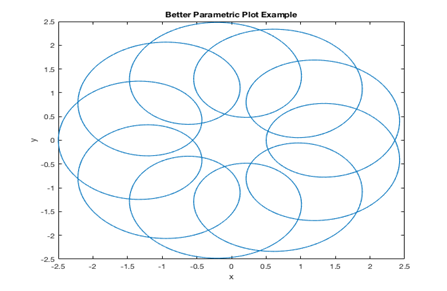
 Parametric plots:

   In a parametric plot, you give both the x and y coordinates of each point as a function of a third parameter, let us consider the parametric example.

r= linspace(0,4*pi,1000)

x=1.5*cos(t)-cos(10*r);

y=1.5*sin®-sin(10*t);

plot(x,y);

x label(‘x’);

y label(‘y’);

title(‘better parametric plot example’)
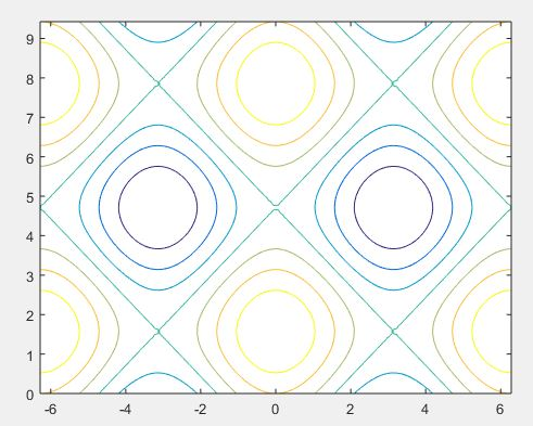
Contour plot:

A contour of a function of two variables may be a curve along which the function features a constant value. Contour lines are used for creating contour maps by joining points of equal elevation above a given level, like mean water level.

A command meshgrid is used to provide grids for the rectangular regions. While the grid used by contour to produce the contour plot for the given region.

a= linspace(-2*pi,2*pi);

b = linspace(0,3*pi);

[a,b] = meshgrid(a,b);

C= cos(a)+sin(b);

contour(a,b,C)

Three dimensional plots:

In three dimensional plots they have three vectors in the same graph (x, y,z) mainly there are five different type of three dimensional plot in matlab. They are;
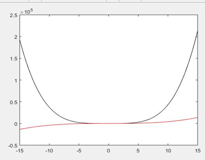
Mesh plot:

The mesh plotting function is employed to display the mesh plot. Which produces an wireframe surface where the lines connecting the defining points are colored.

 [x,y] = meshgrid(-12:0.1:12);

t = sqrt(x.^2+y.^2);

z =(10*sin(t));

mesh(x,y,z)

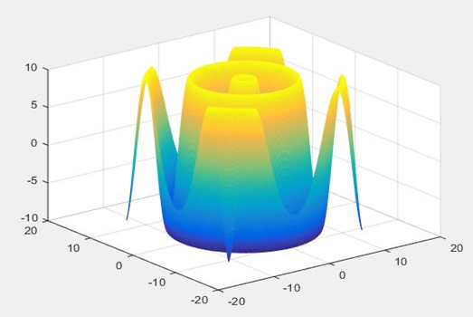
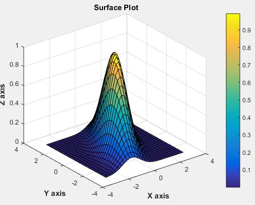
Surface three dimensional plot:

Which is similar to mesh plot main different between them is in surface path the convecting lines and faces will be displayed in dark color. Let us consider the example.

[x,y] = peaks(30);

z = exp(-0.7*(x.^2+0.5*(x-y).^2));

surf(x,y,z);

xlabel(‘\bf X axis’);

ylabel(‘\bf Y axis’);

zlabel(‘\bf Z axis’);

title(‘\bf Surface Plot’)

colorbar

Multiple Functions On the Same Graph

0

Multiple Functions On Same Graph:

In matlab we can draw multiple functions on the same graph by considering some basic colors.

Colors                        code

White                           w

Blue                              b

Cyan                             c

Black                            k

Green                           g

Magenta                       m

Yellow                          y

Red                                r

Let us consider a script for two polynomials.

g(x)= 4x4+3x3+2x2+2x+9

h(x)=4x3+9x+2

x=[-15:0.01:15];

g=4*x.^4 + 3* x.^3 + 2 * x.^2 + 2 * x + 9

h=4 * x.^3 + 9 * x + 2;

Plot(x, g, ‘k’, x, h, ‘r’)

When you run the file you will output as shown in below.

AXIS SETTING:

In order to provide minimum and maximum values for x and y axis by considering the axis command. With axis command allow us to set axis scale.

Syntax will be:

axis ([xmin  xmax  ymin  ymax])

FOR GENERATING SUBPLOT:

Subplot in matlab is used to divide the current figure and allow us to plot multiple figures in the m rows and n column.

Syntax for matlab

Subplot (m, n, p)

Let us consider a example for plotting

In order to plot the income in the top half of the figure and outgo in the bottom half of the figure,

      income = [3.2 4.1 5.0 5.6];
outgo = [2.5 4.0 3.35 4.9];
subplot(2,1,1); plot(income)
subplot(2,1,2); plot(outgo)

Below figure shows four subplot regions

The following combinations produce asymmetrical arrangements of subplots.

 subplot(2,2,[1 3])

subplot(2,2,2)

subplot(2,2,4)

IMPORT, EXPORT DATA IN MATLAB AND PLOTTING

0

IMPORTING DATA:

Where in Matlab importing data is defined as obtaining data from an external file. By using the importing data function we obtain data of different formats with various functions. There are four import functions in Matlab that are described as follows.

C= importdata (format): data from the file named as format is loaded in to the array C.

C=importdata (‘-pastespecial’): loading of records from the system clipboard in place of the document.

C= importdata (___, delimiterIn, headerlinesIn): In this function data is loaded from ASCll file, or clipboard, while the numerical reading starts from line headerlinesIn+1.

C= importdata (___, delimiterIn): In order to separate the column ASCII file or clipboard data we can use delimiterIn.

EXPORT DATA:

In matlab export data means write data in to the file. In matlab there various export data functions, Rectangular, delimited ASCII data file from an array. Diary (or log) document of keystrokes and the ensuing textual content output. Besides from the above there are another way to export a numeric array as a delimited ASCll data file:

With the help of save function we can specify the -ASCII qualifier using the dlmwrite function.

PLOTTING:

In order to plot a graph we use a graph function, to take the following steps:

To draw a graph we should outline the X values from the desired variety for which the graph is plotted.

Let us define the function by considering z=f(x)

Now let’s call plot command, as plot(x,y)

Let us plot simple function y=x for the value in the range of 0 to 200 with an increment in the value of 10.

X= [0:10:200];

z=x;

Plot(x, y)

ADDING TITLE, LABELS AND GRID LINES ON THE GRAPH:

In order to adjust the value in the graph we consider title labels and grid lines. The x label and y label instructions generate labels alongside x-axis and y-axis. The name command permits you to position a name at the graph. The grid on command permits you to position the grid traces at the graph.

concatenating, Determinant of a matrix, String:

0

Concatenating Matrices:

If you concatenate two matrices it creates a large matrix. Pair of square braces [] is a concatenate operator.

Matlab as two types of concatenate as follows:

Horizontal concatenation:

When you concatenate two matrix which are separated by using commas, they are called horizontal concatenation.

Vertical concatenation:

When you concatenate two matrix which are separated by using semicolon, they are called vertical concatenation.

Let us consider an example of this two concatenation:

a = [10 12 15; 14 8 6; 17 8 9]

b = [12 11 45; 8 1 -9; 18 2 11]

 c = [a, b]

d = [a; b]

Output will be obtained as

a= 10 12 15

     14 8 16

     17 8 9

b = 12 31 45

      8 0 -9

      45 2 11

 c = 10 12 15 12 11 45

       14 8   16   8   1 -9

       17 8   9   18 2 11

d=10 12 23

     14 8 6

     27 8 9

   12 31 45

   8 0 -9

   45 2 11

Matrix multiplication:

Where in matrix multiplication, the elements of rows in the first matrix is multiplied with the columns in the second matrix.

In matlab matrix multiplication is represented by ‘*’.

In matrix multiplication column in A matrix is equal to rows in B matrix.

Let us consider an example

a = [2 3 4; 1 2 3; 1 3 5]

b = [2 3 -1; 2 1 3; 5 0 -2;]

prod = a * b

Output will be

prod = 30 9 -1

           21 5 -1

           33 6 -2

Determinant of matrix:

Determinant of matrix is determined by using det function in matlab, and it represented of a matrix A is det(A). Let us consider an example.

a = [ 1 2 6; 2 3 4; 1 4 5]

 det(a)

output will be

ans =17

Inverse of Matrix:

The inverse of a matrix in matlab of A is represented by A−1 such which holds the following relationship:

AA−1 = A−1 A = 1

If the determinant of matrix is zero then the inverse will not exist and the matrix is singular.

Inverse of matrix is determined by inv function in matlab and it represented by inv(A)

STRING:

The string is really a vector whose additives are the numeric codes for the characters. Matlab has exclusive kind of textual content string.

Character array: best when considering individual letters of text, text is stored in two-dimensional array. The rule of all rows should have same number of column.

Cell array: best when considering word.

Let us create an uncomplicated string that may include a unique quote.

msg = ‘You”re right!’

            msg =

You’re right!

create the string, name, the usage of strategies of concatenation.

name = [‘Thomas’ ‘ R. ‘ ‘Lee’]

name = strcat(‘Thomas’,’ R.’,’ Lee’)

Create a vertical array of strings.

C = strvcat (‘Hello’,’Yes’,’No’,’Goodbye’)

C =

Hello 

Yes   

No    

Goodbye

Create a cell array of strings.

S = {‘Hello’ ‘Yes’ ‘No’ ‘Goodbye’}

S =

    ‘Hello’    ‘Yes’    ‘No’    ‘Goodbye’

MATRIX OPERATIONS

0

Deleting row or column in matrix:

An empty braces [] will define the entire row and column of a matrix is deleted. Let us consider an example deleting 2nd row of the:

 a = [3 4 5 6 7; 2 3 4 5 6; 1 2 3 4 5;  4 5 6 7 8];

a ( 2 , : ) = []

if we want to delete the 3rd  column of the given example

a = [2 3 4 5 6; 1 2 3 4 5; 3 4 5 6 7; 4 5 6 7 8];

a(: , 3)=[]

Matrix Operation:

Now let us discuss some commonly used matrix operations are:

Addition and subtraction of matrix:

While performing matrix addition and subtraction when both the operand of matrices must have same number of rows and columns.

Let us consider an example

a = [2 1 3; 4 5 6; 7 8 9];

b = [4 5 6; 1 2 3; 7 8 9];

c = a + b

a = [3 2 4; 4 5 6; 7 8 9];

b = [2 1 3; 3 2 1; 4 5 6];

d = a – b

If we run script file we get:

c= 6 6 9

     5 7 9

     14 16 18

d= 1 1 1

     1 3 5

      3 3 3

Division of (right, left) matrix:

If we want to perform the division of two matrices left (\) or right (/) division operation, when both the operand of matrices must have same number of rows and columns.

Now let us consider an example:

a = [1 2 3; 4 2 6; 7 5 2];

 b = [3 5 6; 2 3 8; 5 7 2];

 c = a / b

d = a \ b

If we run the above example we get output as:

c = -0.7916   0.1666   0.2083

      1.0833   4.3333   0.9166

       2.9583 4.6666   3.8333

 d =

-3.27778   -1.05556   -4.86111

 -0.11111   0.11111   -0.27778

 3.05556      1.27778   4.30556

Transpose of matrix:

The transpose operation will be defined as switching of the rows and columns in a matrix. And it will be represented as a single quote (‘).

Let us consider example:

a = [11 12 13; 14 8 6; 27 8 9]

b = a’

It displayed has:

a = 11 12 13

      14 8   6

      27 8   9

b = 11 14 27

       12 8   8 

       13 6   9

MATLAB ARRAYS

0

Array:

All the variables in matlab are arrays. A scalar is an array with one element, where as a array with one row and one column is called vector. An array with multiple rows and columns is called matrix.

Simply an array of order M x N with a set of number is arranged in a rectangular block of M horizontal rows and N vertical columns.

Creating one dimension array:

 One dimension array defined as numbers are listed in one row and one column, simply known as vector. Then the ith element of a vector k= [k1 k2 k3 k4 … kn]

  Row vector:

    In order to create a row vector provide the space or comma between the elements inside the brackets;

dates = [1     4    10    17    25]

             Or

dates = [1, 4 ,10,17,25]      

Column Vector: In order to create a row vector provide the semicolon between the elements inside the brackets;

Value= [127; 130; 136; 145; 158; 178; 211]

In colon notation, the first number defines the starting values, whereas the second number defines spacing and last number defines ending value.

Value= 2:2:10

Creating a two-dimensional array:

In these the number of rows are equal two number of columns, A matrix is created with the aid of using assigning the elements of the matrix to a variable. This is carried out with the aid of using typing the elements, row with the aid of using row,  within inside the square brackets [ ].

First kind the left bracket [, then type the first row separating the elements with spaces or commas. In order type, the text in the next row types a semicolon or press Enter. Type the right bracket] on the stop of the final row.

VARIABLES IN MATLAB

0

In matlab variables are saved in workspace all through matlab session. While manipulating data at the command line, the variable are stored in base workspace. Variables in workspace can be displayed using whos command. In matlab characteristic has their personal workspace, become independent from matlab workspace.

A Matlab variable is basically which you will assign a value while that value stays in memory. Where the value which was available in the memory so that you can read the programs and operates it on different types of data, and stores back it into memory.

Basically their three types of variables in matlab:

Local Variable:

 A local variable which is described with inside the function. It can only used inside the block code in which it is declared. The local variable exists till the block of the function is below execution. After that, it will be destroyed automatically.

Global Variable:

       A global variable is a program defined outside the function. The scope of global variable, it holds the value through the lifetime of the program.it stores fixed value decided by the complier. Example of global variable:

Function setGlobalx (val)

   global x

   x=val;

end

Persistence Variable:

Persistent variables can be used inside a simplest function only. Persistent variables stay in memory till the M-document is cleared or changed. Persistent is precisely like global, besides that the variable name is not in the global workspace, and the value is reset if the M-document is changed or cleared.

Both the global and local variable are more significant in programming, global variable occupy large memory because of large amount of variables. Therefore, it is beneficial to avoid declaring undesirable global variables.

SWITCH, BREAK, CONTINUE STATEMENTS IN MATLAB

0

SWITCH:

Where in switch case from available number of alternative it execute one set of statement. In this each alternative is considered as a case, switch can handle multiple conditions in a single case statement by enclosing the case expression in a cell array.

This includes the phrase in any other case, observed with the aid of using the statements to execute if the expression’s cost isn’t treated with the aid of using any of the previous case groups.

In its fundamental syntax, switch executes the statements related to the primary case wherein case. When the case expression is a cell array (as with inside the second case above), the case suits if any of the factors of the cell array suits the transfer If no case expression suits the switch expression, then manipulate passes to the in any other case. After the case is executed, application execution resumes with the assertion after the end. If the first case is true then it does not execute next state. So, break statement does not required.

Switch statements

 Case cost1

         Declarations     % executes if statements is cost1

Case cost 1

         Declarations         % executes if statements is cost 2

Otherwise

         Declarations            % executes if statements does not match any case

End

For example let consider to execute a certain block of code based on what the string ‘color’ is set to:

color = ‘rose’;

switch lower(color)
   case {‘red’, ‘light red’, ‘rose’}
      disp(‘color is red’)

   case ‘blue’
      disp(‘color is blue’)

   case ‘white’
      disp(‘color is white’)

   otherwise
      disp(‘Unknown color.’)
end

BREAK:

Break statements is used to exist early from for and while loops. Where in nested loop break is used only for inner loop only, after the execution of the break statement control passes statements that follow the end of that loop. For nested loop if we use break statement only it stop executing inner loop, not outer loop, control passes statements  that follow the end of that loop.

Let’s consider an example:
y = [-2 -4 0 -4 3 7];

% let us test each element with some special condition
for i = 1 : length(z)

   % let we test for the given condition which is  greater-than-zero value
   if z(i) > 0
      %  let we terminates the loop execution
      break
   end
   y = z(i) + 5;
   disp(y)
  
end

CONTINUE:

Continue statement temporary interrupts the program execution loop, skipping any given remaining statements in the body of the loop and continues with the current pass. Let’s consider an example. % Let’s us consider an example and execute the example based on assumption that you are verifying a set of values.
for i = 1: 9
if (i == 2 | i == 3)
    continue
end

  % here we can continue with the remaining values,
  disp (i)

end

Loops In Matlab

0

FLOW CONTROL AND LOOPS (ITERATION):

Loop or iteration are useful for execution of the sequence more than once of the given statements. Basically their two types of loop forms they are: while loops and for loops. Main different between these two loops is how repetition took place in both while and for loops. While loop is used when how many times you want the loop to execute it is done based on the given condition. When going to for loop the number of repetition are given before the loop start execution.

WHILE LOOP:  

While loop executes the group of statements are statement indefinite number of times until the logic condition become true. Syntax of while loop:

         While expression

                Statements

            end

For example, suppose you wanted to double the number 2 over and over again until you got to a number over 1,000,000

           number = 2;

           counter = 1;

    while number <= 10^6

                number = 2*number;

               counter = counter + 1;

      end

FOR LOOP:

For loop is used for execution of group of statements or a statement for predefined number of times. Syntax of for loop.

        For index = start: increment: end

           Statements

       End

Where index is the loop control variable

For example

    s = 0;

   For i = 1:10 %increment of 1

        s = s + i;

  End

 disp(s);

FLOW CONTROL:

IF, ELSE AND ELSEIF:

If statements evaluate the logical expression and execute the group of statements when the expression is true, otherwise for execution of alternate statements it go with else or else if. An end keyword, which matches the if, terminates the last group of statements. If the logical expression is true (1), MATLAB executes all the statements between the if and end lines. It resumes execution at the line following the end statement. If the condition is false (0), MATLAB skips all the statements between the if and end lines, and resumes execution at the line following the end statement. Syntax of if condition.

if logical_expression

 Statements

 End

The else if statement has a logical condition that it evaluates if the preceding if (and possibly elseif condition) is false (0). The statements associated with it execute if its logical condition is true (1). You can have multiple elseifs within an if block. Syntax of elseif condition.

if expression

    Statements

elseif expression

    Statements

else

    Statements

end

           x = rand;

            if x < 1/3

              disp(‘x < 1/3’);

             else if x < 2/3

                     disp(‘1/3 <= x < 2/3’);

              else

                   disp(‘2/3 <= x ’);

             end

BIT-WISE OPERATOR And SHORT CIRCUIT OPERATOR

0

BIT-WISE OPERATOR:

In bit-wise operator logical bit-wise operation is performed for positive integer input, where the input may be scalar or array. Below shows some functions of bit-wise operator.

Bitand       it performs the bit-wiseAnd operation on two positive integers.

For example: A = 28;         % binary 11100
                  B = 21;         % binary 10101

bitand (A, B) = 20
(binary 10100)

Bitor          it performs the bit-wiseor operation on two positive integers.

For example: A = 28;         % binary 11100
                  B = 21;         % binary 10101

bitor(A,B) = 29
(binary 11101)

Bitcmp   It returns the bit-wise complement as an n-bit number, where n is the second input argument to bitcmp.

    For example: A = 28;         % binary 11100
                  B = 21;         % binary 10101

bitcmp(A,5) = 3
(binary 00011)

Bitxor      It returns the bit-wise exclusive OR of two nonnegative integer arguments.

                                  For example: A = 28;         % binary 11100
                                                        B = 21;         % binary 10101

Bitxor (A,B) = 9
(binary 01001)

SHORT CIRCUIT OPERATOR:

 Short-circuit operator used when first operand does not determine the output fully we consider the short-circuiting operator to calculate the second operand.

&& It returns logical 1 (true) if both inputs calculate to true, and logical 0 (false) if they do not.


|| It returns logical 1 (true) if either input, or both, calculate to true, and logical 0 (false) if they do not.

RELATIONAL OPERATOR:

Relational operator performs element by element comparison between two arrays. They return a logical array of the identical size.

A < B                  A Less than B
A > B                  A Greater than B

A <= B                 A Less than or equal to B

C >= D                C Greater than or equal to D
A == B                 A Equal to B
A ~= B                 A Not equal to B