BASIC OPERATIONS ON SIGNALS:
When we perform an operation signal it may undergoes several manipulation which may include amplitude of the signal or independent variable. Some basic operation are performed on signals. They are:
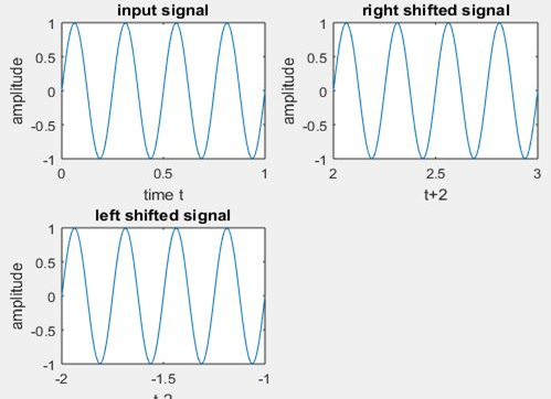
Time-shifting:
Time shifting of a signal x(n) may be defined as delay or advance of a signal in time, which is represented with the function.
y(n)=x(n+k)
When k is positive, then y(n) is shifted to right then the signal is delayed, when y(n) is shifted to left then the signal is advanced.
clc;
close all;
clear all;
t=0:.01:1;
x1=sin(2*pi*4*t);
%shifting of a signal 1
figure;
subplot(2,2,1);
plot(t,x1);
xlabel(‘time t’);
ylabel(‘amplitude’);
title(‘input signal’);
subplot(2,2,2);
plot(t+2,x1);
xlabel(‘t+2’);
ylabel(‘amplitude’);
title(‘right shifted signal’);
subplot(2,2,3);
plot(t-2,x1);
xlabel(‘t-2’);
ylabel(‘amplitude’);
title(‘left shifted signal’);
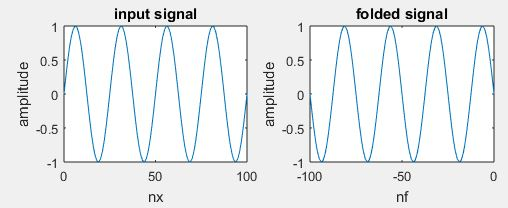
Time reversal:
Time reversal of a signal x(t) is defined as folding of a signal at t=0,it is very useful in convolution.
Y(t)=y(-t)
clc;
close all;
clear all;
t=0:.01:1;
x1=sin(2*pi*4*t);
h=length(x1);
nx=0:h-1;
subplot(2,2,1);
plot(nx,x1);
xlabel(‘nx’);
ylabel(‘amplitude’);
title(‘input signal’)
y=fliplr(x1);
nf=-fliplr(nx);
subplot(2,2,2);
plot(nf,y);
xlabel(‘nf’);
ylabel(‘amplitude’);
title(‘folded signal’);
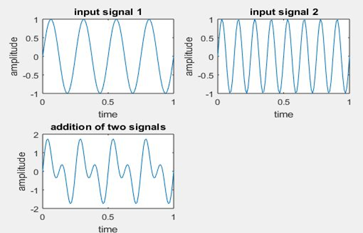
Addition:
Addition of signal may be defined as adding of two continuous signals x1(t) and x2(t) at every time instant.
c(t) = x (t) + y (t)
clc;
close all;
clear all;
t=0:.01:1;
x1=sin(2*pi*4*t);
x2=sin(2*pi*8*t);
subplot(2,2,1);
plot(t,x1);
xlabel(‘time’);
ylabel(‘amplitude’);
title(‘input signal 1’);
subplot(2,2,2);
plot(t,x2);
xlabel(‘time’);
ylabel(‘amplitude’);
title(‘input signal 2’);
y1=x1+x2;
subplot(2,2,3);
plot(t,y1);
xlabel(‘time’);
ylabel(‘amplitude’);
title(‘addition of two signals’);
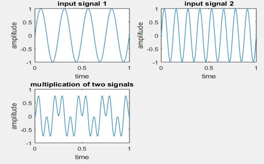
Multiplication:
Multiplcation of signal may be defined as multiplying of two continuous signals x1(t) and x2(t) at every time instant.
C(t)=x(t) y(t)
clc;
close all;
clear all;
t=0:.01:1;
x1=sin(2*pi*4*t);
x2=sin(2*pi*8*t);
subplot(2,2,1);
plot(t,x1);
xlabel(‘time’);
ylabel(‘amplitude’);
title(‘input signal 1’);
subplot(2,2,2);
plot(t,x2);
xlabel(‘time’);
ylabel(‘amplitude’);
title(‘input signal 2’);
y2=x1.*x2;
subplot(2,2,3);
plot(t,y2);
xlabel(‘time’);
ylabel(‘amplitude’);
title(‘multiplication of two signals’);
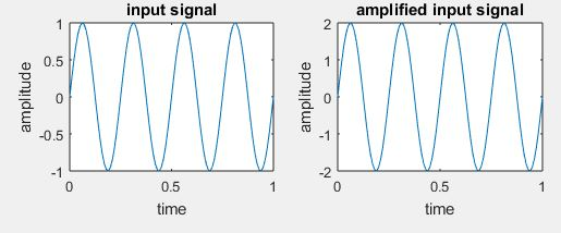
Scaling:
Scaling is defined as time expansion are compression of a given signal. Mathematically is represented as
Y(t)=x(at)
clc;
close all;
clear all;
t=0:.01:1;
x1=sin(2*pi*4*t);
A=2;
y=A*x1;
figure;
subplot(2,2,1);
plot(t,x1);
xlabel(‘time’);
ylabel(‘amplitude’);
title(‘input signal’)
subplot(2,2,2);
plot(t,y);
xlabel(‘time’);
ylabel(‘amplitude’);
title(‘amplified input signal’);