In matlab variables are saved in workspace all through matlab session. While manipulating data at the command line, the variable are stored in base workspace. Variables in workspace can be displayed using whos command. In matlab characteristic has their personal workspace, become independent from matlab workspace.

A Matlab variable is basically which you will assign a value while that value stays in memory. Where the value which was available in the memory so that you can read the programs and operates it on different types of data, and stores back it into memory.

Basically their three types of variables in matlab:

Local Variable:

 A local variable which is described with inside the function. It can only used inside the block code in which it is declared. The local variable exists till the block of the function is below execution. After that, it will be destroyed automatically.

Global Variable:

       A global variable is a program defined outside the function. The scope of global variable, it holds the value through the lifetime of the program.it stores fixed value decided by the complier. Example of global variable:

Function setGlobalx (val)

   global x

   x=val;

end

Persistence Variable:

Persistent variables can be used inside a simplest function only. Persistent variables stay in memory till the M-document is cleared or changed. Persistent is precisely like global, besides that the variable name is not in the global workspace, and the value is reset if the M-document is changed or cleared.

Both the global and local variable are more significant in programming, global variable occupy large memory because of large amount of variables. Therefore, it is beneficial to avoid declaring undesirable global variables.

SWITCH:

Where in switch case from available number of alternative it execute one set of statement. In this each alternative is considered as a case, switch can handle multiple conditions in a single case statement by enclosing the case expression in a cell array.

This includes the phrase in any other case, observed with the aid of using the statements to execute if the expression’s cost isn’t treated with the aid of using any of the previous case groups.

In its fundamental syntax, switch executes the statements related to the primary case wherein case. When the case expression is a cell array (as with inside the second case above), the case suits if any of the factors of the cell array suits the transfer If no case expression suits the switch expression, then manipulate passes to the in any other case. After the case is executed, application execution resumes with the assertion after the end. If the first case is true then it does not execute next state. So, break statement does not required.

Switch statements

 Case cost1

         Declarations     % executes if statements is cost1

Case cost 1

         Declarations         % executes if statements is cost 2

Otherwise

         Declarations            % executes if statements does not match any case

End

For example let consider to execute a certain block of code based on what the string ‘color’ is set to:

color = ‘rose’;

switch lower(color)
   case {‘red’, ‘light red’, ‘rose’}
      disp(‘color is red’)

   case ‘blue’
      disp(‘color is blue’)

   case ‘white’
      disp(‘color is white’)

   otherwise
      disp(‘Unknown color.’)
end

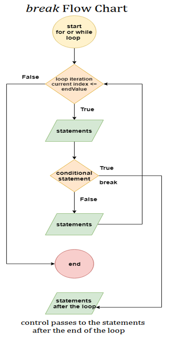
BREAK:

Break statements is used to exist early from for and while loops. Where in nested loop break is used only for inner loop only, after the execution of the break statement control passes statements that follow the end of that loop. For nested loop if we use break statement only it stop executing inner loop, not outer loop, control passes statements  that follow the end of that loop.

Let’s consider an example:
y = [-2 -4 0 -4 3 7];

% let us test each element with some special condition
for i = 1 : length(z)

   % let we test for the given condition which is  greater-than-zero value
   if z(i) > 0
      %  let we terminates the loop execution
      break
   end
   y = z(i) + 5;
   disp(y)
  
end

CONTINUE:

Continue statement temporary interrupts the program execution loop, skipping any given remaining statements in the body of the loop and continues with the current pass. Let’s consider an example. % Let’s us consider an example and execute the example based on assumption that you are verifying a set of values.
for i = 1: 9
if (i == 2 | i == 3)
    continue
end

  % here we can continue with the remaining values,
  disp (i)

end

FLOW CONTROL AND LOOPS (ITERATION):

Loop or iteration are useful for execution of the sequence more than once of the given statements. Basically their two types of loop forms they are: while loops and for loops. Main different between these two loops is how repetition took place in both while and for loops. While loop is used when how many times you want the loop to execute it is done based on the given condition. When going to for loop the number of repetition are given before the loop start execution.

WHILE LOOP:  

While loop executes the group of statements are statement indefinite number of times until the logic condition become true. Syntax of while loop:

         While expression

                Statements

            end

For example, suppose you wanted to double the number 2 over and over again until you got to a number over 1,000,000

           number = 2;

           counter = 1;

    while number <= 10^6

                number = 2*number;

               counter = counter + 1;

      end

FOR LOOP:

For loop is used for execution of group of statements or a statement for predefined number of times. Syntax of for loop.

        For index = start: increment: end

           Statements

       End

Where index is the loop control variable

For example

    s = 0;

   For i = 1:10 %increment of 1

        s = s + i;

  End

 disp(s);

FLOW CONTROL:

IF, ELSE AND ELSEIF:

If statements evaluate the logical expression and execute the group of statements when the expression is true, otherwise for execution of alternate statements it go with else or else if. An end keyword, which matches the if, terminates the last group of statements. If the logical expression is true (1), MATLAB executes all the statements between the if and end lines. It resumes execution at the line following the end statement. If the condition is false (0), MATLAB skips all the statements between the if and end lines, and resumes execution at the line following the end statement. Syntax of if condition.

if logical_expression

 Statements

 End

The else if statement has a logical condition that it evaluates if the preceding if (and possibly elseif condition) is false (0). The statements associated with it execute if its logical condition is true (1). You can have multiple elseifs within an if block. Syntax of elseif condition.

if expression

    Statements

elseif expression

    Statements

else

    Statements

end

           x = rand;

            if x < 1/3

              disp(‘x < 1/3’);

             else if x < 2/3

                     disp(‘1/3 <= x < 2/3’);

              else

                   disp(‘2/3 <= x ’);

             end

BIT-WISE OPERATOR:

In bit-wise operator logical bit-wise operation is performed for positive integer input, where the input may be scalar or array. Below shows some functions of bit-wise operator.

Bitand       it performs the bit-wiseAnd operation on two positive integers.

For example: A = 28;         % binary 11100
                  B = 21;         % binary 10101

bitand (A, B) = 20
(binary 10100)

Bitor          it performs the bit-wiseor operation on two positive integers.

For example: A = 28;         % binary 11100
                  B = 21;         % binary 10101

bitor(A,B) = 29
(binary 11101)

Bitcmp   It returns the bit-wise complement as an n-bit number, where n is the second input argument to bitcmp.

    For example: A = 28;         % binary 11100
                  B = 21;         % binary 10101

bitcmp(A,5) = 3
(binary 00011)

Bitxor      It returns the bit-wise exclusive OR of two nonnegative integer arguments.

                                  For example: A = 28;         % binary 11100
                                                        B = 21;         % binary 10101

Bitxor (A,B) = 9
(binary 01001)

SHORT CIRCUIT OPERATOR:

 Short-circuit operator used when first operand does not determine the output fully we consider the short-circuiting operator to calculate the second operand.

&& It returns logical 1 (true) if both inputs calculate to true, and logical 0 (false) if they do not.

|| It returns logical 1 (true) if either input, or both, calculate to true, and logical 0 (false) if they do not.

RELATIONAL OPERATOR:

Relational operator performs element by element comparison between two arrays. They return a logical array of the identical size.

A < B                  A Less than B

A > B                  A Greater than B

A <= B                 A Less than or equal to B

C >= D                C Greater than or equal to D

A == B                 A Equal to B

A ~= B                 A Not equal to B