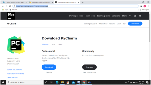
Installation of PyCharm IDE
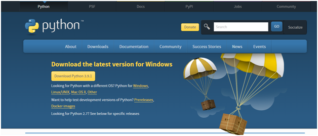
- Navigate to official Pycharm websitehttps://www.jetbrains.com/pycharm..\Downloads\latest and download Pycharm .
- Run the exe file to Install PyCharm and you can also install PyCharm on windows manually by configuring PyCharm location on your c drive or change location of PyCharm .
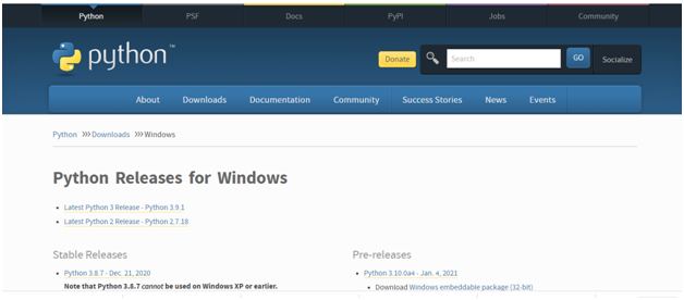
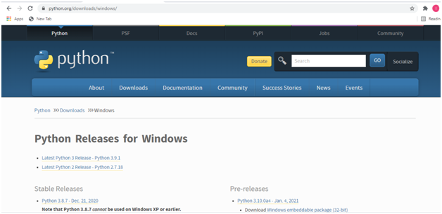
- You can effortlessly configure PyCharm on windows 10 and to code in python you need to install PyCharm in windows 10 depending up on your system compatibility if its 32 but 0r 64 bit.
- PyCharm is not only the IDE through which you can execute python code in windows 10 but PyCharm is the most widely used IDE or integrated development environment for Python & compatable and will execute complex python code easily.
- PyCharm is accesable in three editions Professional, Community, and Edu. It offers to download in 32 bit and 62 bit for windows 10 and also you can install pycharm on your mac by downloading .dmg file.
How to install Pycharm on Windows
The following is the step by step procedure to install Pycharm in windows 10
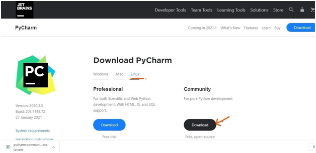
- To download and install Pycharm go to the official website https://www.jetbrains.com/pycharm.
- Download the community version
Install the downloaded file.
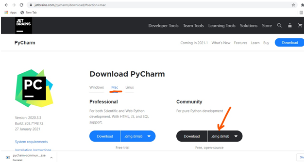
How to install Pycharm in Mac?
The following is the step by step procedure to install Pycharm for Mac
- Navigate to the official website and download the .dmg file.
- Install the downloaded file.
How to install Pycharm in Linux?
1. Go to the official website of Pycharm
2. click on the Linux OS and download.
3. Install the downloaded file.