TO PLOT POLES AND ZEROS OF THE GIVEN TRANSFORM FUNCTION

Z TRANSFORM

 For discrete time linear time-invariant system with impulse response h[n], the response y[n] of the system to a complex exponential input of the form z^-1 is

Y[n] =H[z].zⁿ

Where H[z] =  zⁿ                  ——-2

For z=e^jw with  real (i.e., with |z| =1), the sum in above equation corresponds to the discrete-time Fourier transform of h[n].

Generally, when |z| is not restricted to unity, then summation in equation 2 is referred as z transform of h[n].

Z transform for the discrete time signal x[n] is determined as

X[z] =  zⁿ          

Where, z= a complex variable.

Program:

clc;

clear all;

close all;

%enter the numerator and denominators coefficients in square brackets

num=input(‘enter numerator co-efficients’);

den=input(‘enter denominator co-efficients’);

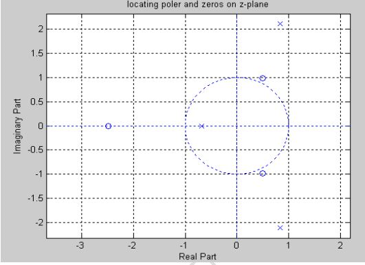
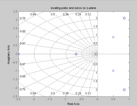
% find poles and zeros

poles=roots(den)

zeros=roots(num)

% find transfer function H(s)

h=tf(num,den);

% plot the pole-zero map in s-plane

sgrid;

pzmap(h);

grid on;

title(‘locating poles and zeros on s-plane’);

%plot the pole zero map in z-plane

figure

zplane(poles,zeros);

grid on;

title(‘locating poles and zeros on z-plane’);

Output:

Enter numerator co-efficients [2 -12 4 5]

Enter denominator co-efficients [3 4 5 6]

Poles =

  -1.2653 + 0.0000i

  -0.0340 + 1.2568i

  -0.0340 – 1.2568i

Zeros =

    5.5594

    0.9262

   -0.4855

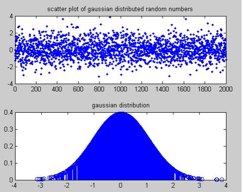
• GAUSSIAN NOISE:

Gaussian noise will be defined as statistical noise which features a probability density function of the traditional distribution (also referred to as Gaussian distribution). In other words, the valuestha the noise can combat are Gaussian-distributed. It is most ordinarily used as additive noise to yield additive white Gaussian noise (AWGN). Gaussian noise is correctly defined because of the noise with a Gaussian amplitude distribution.

Program:

clc;

clear all;

close all;

%let’s generates the given set of 2000 samples for Gaussian distributed random numbers

x=randn(1,2000);

%to plot the joint distribution for both the sets using dot.

subplot(211)

plot(x,’.’);

title(‘scatter plot of gaussian distributed random numbers’);

ymu=mean(x);

ymsq=sum(x.^2)/length(x);

ysigma=std(x);

yvar=var(x);

yskew=skewness(x);

p=normpdf(x,ymu,ysigma);

subplot(212);

stem(x,p);

title(‘ gaussian distribution’);