Wiener-Khinchin:
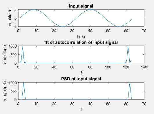
The Wiener-Khinchin theorem is a fundamental theorem useful for the stochastic processes. The Wiener-Khinchin theorem provides a simple relationship between time and frequency representations of a fluctuating process. Its great practical importance comes from the fact that the autocorrelation function may be directly determined from the measured power spectral density, and vice versa. The wiener-Khinchin is widely used theorem to states the power spectral density of a wide sense stationary random process of the flourier transform for the corresponding autocorrelation function.
Program:
clc;
clear all;
close all;
t=0:0.1:2*pi;
%input signal
x=sin(2*t);
subplot(3,1,1);
plot(x);
xlabel(‘time’);
ylabel(‘amplitude’);
title(‘input signal’);
%autocorrelation of input signal
xu=xcorr(x,x);
%fft of autocorrelation signal
y=fft(xu);
subplot(3,1,2);
plot(abs(y));
xlabel(‘f’);
ylabel(‘amplitude’);
title(‘fft of autocorrelation of input signal’);
%fourier transform of input signal
y1=fft(x);
%finding the power spectral density
y2=(abs(y1)).^2;
subplot(3,1,3);
plot(y2);
xlabel(‘f’);
ylabel(‘magnitude’);
title(‘PSD of input signal’);
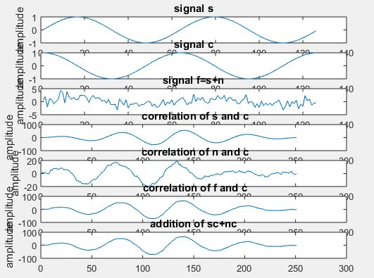
Extraction Of Periodic Signal Using Correlation:
A signal is masked by noise are often detected either by correlation techniques or by filtering. Actually, the two techniques are equivalent. The correlation technique may be a measure of extraction of a given signal within the time domain whereas filtering achieves precisely the same leads to frequency domain.
Program:
clear all;
close all;
clc;
t=0:0.1: pi*4;
%input signal1
s=sin(t);
subplot(7,1,1)
plot(s);
title(‘signal s’);
xlabel(‘t’);
ylabel(‘amplitude’);
%input signal2
c=cos(t);
subplot(7,1,2)
plot(c);
title(‘signal c’);
xlabel(‘t’);
ylabel(‘amplitude’);
%generating noise signal
n = randn([1 126]);
%signal+noise
f=s+n;
subplot(7,1,3);
plot(f);
title(‘signal f=s+n’);
xlabel(‘t’);
ylabel(‘amplitude’);
%cross correlation of signal1&signal2
asc=xcorr(s,c);
subplot(7,1,4)
plot(asc);
title(‘ correlation of s and c’);
xlabel(‘t’);
ylabel(‘amplitude’);
%cross correlation of noise&signal2
anc=xcorr(n,c);
subplot(7,1,5)
plot(anc);
title(‘ correlation of n and c’);
xlabel(‘t’);
ylabel(‘amplitude’);
%cross correlation of f&signal2
cfc=xcorr(f,c);
subplot(7,1,6)
plot(cfc);
title(‘ correlation of f and c’);
xlabel(‘t’);
ylabel(‘amplitude’);
%extracting periodic signal
hh=asc+anc;
subplot(7,1,7)
plot(hh);
title(‘addition of sc+nc’);
xlabel(‘t’);
ylabel(‘amplitude’);