| Conventional mobile Systems | Cellular mobile system |
| Spectrum utilization is inefficient in conventional mobile system since each channel serves only one customer at a time. | The cellular system improves efficiency by three approaches The allocated frequency band is divided into maximum number off channels The allocated frequency band is reused in different geographic locations.Using Spread spectrum or frequency hopped technique, many codes are generated over a wide frequency band. |
| Conventional mobile telephone systems use single carrier frequency leading to half duplex .i.e., one way communication. | Cellular mobile phones provides full duplex i.e., two way communication |
| Conventional Mobile systems use a high power transmitters to cover large areas | Cellular mobile system uses low power transmitters to cover the same area. |
| Conventional mobile systems experiences the problem like spectral congestion and user capacity. | Cellular system solves this problem by providing high user capacity relatively within the limited spectrum of frequency. |
| Conventional systems are not widely used due to its high cost and limited availability. | Cellular systems offer more availability and low cost. |
| Conventional systems cover only a smaller area. | Cellular systems cover large area. |
| In conventional system, the capacity is increased by increasing RF. | In mobile system, the mobile unit capacity is maximized without increasing RF. |
| Conventional systems do not maintain privacy. | Cellular systems maintain privacy. |
Advantages of Cellular systems over conventional mobile systems

Introduction to Cellular Concept
Cellular Concept:
- Cellular concept deals with reduction of service area by employing high power transmitters that offer high capacity in a limited spectrum allocation.
- In a geographic region, each base station is assigned with different group of channels from the total number of channels available to the entire system.
- This distribution cochannels reduce the interference between the base stations and mobile users under their control.
- The channels can be reused until the interference between cochannel stations is at acceptable level.
- The number of base stations increase with increase in demand for service, hence, providing additional radio capacity within the radio spectrum.
- Cellular concept is responsible for manufacturing every piece of user equipment of large area such that any mobile can be accessed within the range.
Advantages of cellular system:
- Problem of spectral congestion is solved by cellular system.
- It offers high capacity with limited spectrum.
- This high capacity is achieved by limiting the coverage area of each base station to a small geographic area termed as cell.
- In cellular system each high power transmitter is replaced with several low power transmitters.
- Each base station is allocated a portion of channels and nearby cells are allocated completely different channels.
- All available channels are allocated to small number of base stations.
Cell parameters and signal strength
The cellular system depends on the radio signal received by a mobile station throughout the cell and on the contours of signal strength emanating from the base station of two adjacent cells j and i.
As from the above discussion, the signal strength goes down as moves away from the base station. The difference in received power is a function of distance. Whereas the mobile station moves away from the base station of the cell, the signal strength weakness, and at some point, a phenomenon known as handoff occurs. This implies a radio connection to another adjacent cell. j
As the mobile station moves away from j cell and gets closer to the cell i. assuming that pj(x) and pi(y) represents the power received at the mobile station from the BSj and BSi, the received signal strength at the mobile station can be represented by curves and the variation can be expressed by the empirical relations. While the distance X1 from the received signal of BSj is approximately close to zero and the signal strength at the mobile station can be primarily attributed to BSi. While, at distance X2, the signal from BSi is minor. To receive and interpret the signals correctly at the mobile station, the received signal must be at a given minimum power level pmin and the distance X3 and X4 have two such points for BSj and BSi, respectively.
Therefore that, between points X3 and X4, the mobile station is going to be served by either BSj and BSi, and therefore the choice is left to the service provider and the underlying technology. where the mobile station have a radio link with BSj and continuously moving towards away BSi then at some point it has to be connected to the BSi and the change of such linkage from BSj to BSi is known as a handoff. Therefore regions X3 and X4 indicate the handoff area.
Where the performs handoff depends on many factors.One of the considerations is that the handoff should not take place too quickly to make the MS change the BS too frequently. If the Mobile station moves forth and back between the overlapped area of two adjacent cells due to underlying terrain or intentional movements.
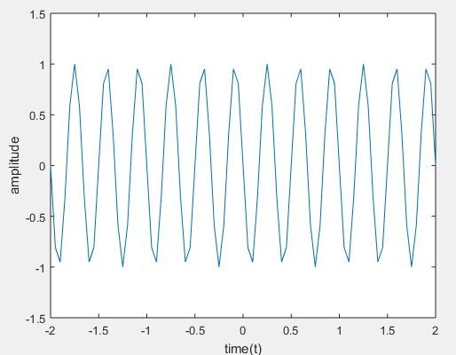
DTMF SIGNAL GENERATION

The DTMF stands for “Dual Tone Multi-Frequency”, and maybe a method of representing digits with tone frequencies, so as to transmit them over an analog communications network, for instance, a telephone line. In telephone networks, DTMF signals are wont to encode dial trains and other information. Dual-tone Multi-Frequency (DTMF) signaling is widely used for voice communications control and is mostly used worldwide in modern telephony to configure switchboards and to dial numbers. It is also utilized in systems like voice mail, electronic message, and telephone banking. The DTMF signal is considered as the sum of two sinusoids – or tones – with frequencies taken from two mutually exclusive groups. Where these frequencies are chosen to stop any harmonics from being incorrectly detected by the receiver as another DTMF frequency. while each pair of tones consist of one set frequency of the low group (697 Hz, 770 Hz, 852 Hz, 941 Hz) and another set frequency of the high group ( 1336 Hz, 1477Hz,1209 Hz) and represents a unique symbol.
Program:
clc;
clear all;
close all;
t = -2:0.05:2;
x=input(‘enter the input number’);
fr1=697;
fr2=770;
fr3=852;
fr4=941;
fc1=1209;
fc2=1336;
fc3=1477;
fc4=1633;
y0 = sin(2*pi*fr4*t) + sin(2*pi*fc2*t); % 0
y1 = sin(2*pi*fr1*t) + sin(2*pi*fc1*t); % 1
y2 = sin(2*pi*fr1*t) + sin(2*pi*fc2*t); % 2
y3 = sin(2*pi*fr1*t) + sin(2*pi*fc3*t); % 3
y4 = sin(2*pi*fr2*t) + sin(2*pi*fc1*t); % 4
y5 = sin(2*pi*fr2*t) + sin(2*pi*fc2*t); % 5
y6 = sin(2*pi*fr2*t) + sin(2*pi*fc3*t); % 6
y7 = sin(2*pi*fr3*t) + sin(2*pi*fc1*t); % 7
y8 = sin(2*pi*fr3*t) + sin(2*pi*fc2*t); % 8
y9 = sin(2*pi*fr3*t) + sin(2*pi*fc3*t); % 9
y_start = sin(2*pi*fr4*t) + sin(2*pi*fc1*t); % *
y_canc = sin(2*pi*fr4*t) + sin(2*pi*fc3*t); % #
if (x==1)
plot(t,y1)
xlabel(‘time(t)’)
ylabel(‘amplitude’)
elseif (x==2)
plot(t,y2)
xlabel(‘time(t)’)
ylabel(‘amplitude’)
elseif (x==3)
plot(t,y3)
xlabel(‘time(t)’)
ylabel(‘amplitude’)
elseif (x==4)
plot(t,y4)
xlabel(‘time(t)’)
ylabel(‘amplitude’)
elseif (x==5)
plot(t,y5)
xlabel(‘time(t)’)
ylabel(‘amplitude’)
elseif (x==6)
plot(t,y6)
xlabel(‘time(t)’)
ylabel(‘amplitude’)
elseif (x==7)
plot(t,y7)
xlabel(‘time(t)’)
ylabel(‘amplitude’)
elseif (x==8)
plot(t,y8)
xlabel(‘time(t)’)
ylabel(‘amplitude’)
elseif (x==9)
plot(t,y9)
xlabel(‘time(t)’)
ylabel(‘amplitude’)
elseif (x==0)
plot(t,y0)
xlabel(‘time(t)’)
ylabel(‘amplitude’)
elseif (x==11)
plot(t,y_start)
xlabel(‘time(t)’)
ylabel(‘amplitude’)
elseif (x==12)
plot(t,y_canc)
xlabel(‘time(t)’)
ylabel(‘amplitude’)
else
disp(‘enter the correct input’)
end
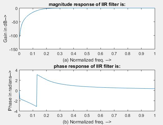
Low pass IIR filter implementation
Where has IIR filters are digital filters with infinite impulse response. Unlike FIR filters, they have the feedback (a recursive a part of a filter) and are mentioned as recursive digital filters, therefore. For this reason, IIR filters have far better frequency responses than FIR filters of an equivalent order. Unlike FIR filters, their phase characteristic isn’t linear which may cause a drag to the systems which require phase linearity. For this reason, it isn’t preferable to use IIR filters in digital signal processing when the phase is of the essence. Otherwise, when the linear phase characteristic isn’t important, that is typical of IIR filters only. FIR filters don’t have such a drag as they are doing not have the feedback. For this reason, it’s always necessary to see after the planning process whether the resulting IIR filter is stable or not.
IIR FILTER DESIGN
For the given specifications to style a digital IIR filter, first we’d like to style analog filter (Butterworth or chebyshev). The resultant analog filter is transformed to digital filter by using either “Bilinear transformation or Impulse Invariant transformation”
Steps for performing IIR filter
Step I: while enter the pass band ripple (rp) and stop band ripple (rs).
Step II: Let’s enter the pass band frequency (wp) and stop band frequency (ws).
Step III: After we get the sampling frequency (fs).
Step IV: Next calculate normalized pass band frequency, and normalized stop band frequency w1 and w2 respectively.
Step V :And make use of the following function to calculate order of filter Butterworth filter order [n,wn]=buttord(w1,w2,rp,rs ) Chebyshev filter order [n,wn]=cheb1ord(w1,w2,rp,rs)
Step VI : Let’s Design an nth order digital low pass Butterworth or Chebyshev filter using the following statements. Butterworth filter [b, a]=butter (n, wn) Chebyshev filter [b,a]=cheby1 (n, 0.5, wn)
Step VII : To find the digital frequency response of the filter by using ‘freqz( )’ function
Step VIII : Next calculate the magnitude of the frequency response in decibels (dB) mag=20*log10 (abs (H))
Step IX : To plot the magnitude response [magnitude in dB Vs normalized frequency]
Step X : And calculate the phase response using angle (H) S
Step XI : To plot the phase response [phase in radians Vs normalized frequency (Hz)].
Program:
clc;
clear all;
close all;
disp(‘enter the IIR filter design specifications’);
rp=input(‘enter the passband ripple’);
rs=input(‘enter the stopband ripple’);
wp=input(‘enter the passband freq’);
ws=input(‘enter the stopband freq’);
fs=input(‘enter the sampling freq’);
w1=2*wp/fs;w2=2*ws/fs;
[n,wn]=buttord(w1,w2,rp,rs,’s’);
disp(‘Frequency response of IIR HPF is:’);
[b,a]=butter(n,wn,’high’,’s’);
w=0:.01:pi;
[h,om]=freqs(b,a,w);
m=20*log10(abs(h));
an=angle(h);
figure, subplot(2,1,1);plot(om/pi,m);
title(‘magnitude response of IIR filter is:’);
xlabel(‘(a) Normalized freq. –>’);
ylabel(‘Gain in dB–>’);
subplot(2,1,2);plot(om/pi,an);
title(‘phase response of IIR filter is:’);
xlabel(‘(b) Normalized freq. –>’);
ylabel(‘Phase in radians–>’);
output:
enter the IIR filter design specifications
enter the passband ripple13
enter the stopband ripple50
enter the passband freq1200
enter the stopband freq250
enter the sampling freq6000
CELLULAR SYSTEM
Fundamental concept of cellular system:
Let see example of cordless telephone used at home which employed wireless technology, which has less coverage and smaller amount of power. All the users use same frequency range without much inference among users. Same frequency interference avoidance is used in cellular system with much more powerful transmitting station, or base station.
Introduction to cellular concept:
A cell is defined as the use of mobile station radio communication resources is under the control of the base station. Depending on the size, shape and amount of resources allocated to each cell determines the performance of the system.
Cell area:
The important factor in the cellular system is the size and shape of the cell. Transmitter or base station coverage area is called a cell, base station serve all the mobile station connected to it in that area. Whereas the coverage area of the base station can be represented by a cellular cell with a radius R from the center of the base station. While the many factors affecting the signal strength including refraction of the signal, reflection, elevation of the terrain due to the presence of tall buildings or valleys, or hills. Received signal strength will determine the original shape of the cell. Cell boundaries are represented by using different models are hexagon, square, and equilateral triangle. From the available model hexagon mostly used model due to its arrangement style. In a hexagon, multiple hexagons is arranged next to each other, without having any spacing between two hexagons without any overlapping area. Another most popular model is a rectangular shape, which is similar to the hexagon model. If the cell area is increased the number of the channels per unit area is reduced for the same number of channels and if the populated area is less it is good which has fewer subscribers.
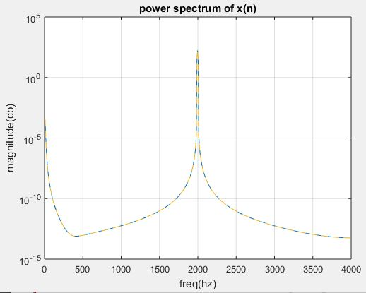
POWER SPECTRUM DETERMINATION OF GIVEN SIGNAL AND LOWPASS FIR FILTER IMPLEMENTATION
POWER SPECTRUM DETERMINATION OF GIVEN SIGNAL
THEORY: The power spectrum describes the distribution of signal power over a frequency spectrum. The most frequently used way of generating a power spectrum is with using a discrete Fourier transform, but also other techniques such as the maximum entropy method can also be used. The power spectrum also can be defined because the Fourier transform of auto correlation function.
Steps involved in performing power spectrum operation for a given signal
Step I: let’s consider input sequence x
Step II: And the given sampling frequency, input frequency and length of the spectrum.
Step III: In order to find power spectrum of input sequence by using matlab command spectrum.
Step IV: And plot power spectrum using specplot.
Program:
clc;
clear all;
close all;
N=1024;
fs=8000;
f=input(‘enter the frequency[1 to 5000]:’);
n=0:N-1;
x=sin(2*pi*(f/fs)*n)
pxx=spectrum(x,N);
specplot(pxx,fs);
grid on
xlabel(‘freq(hz)’);
ylabel(‘magnitude(db)’);
title(‘power spectrum of x(n)’);
Enter the frequency [1 to 5000]:2000
LOWPASS FIR FILTER IMPLEMENTATION
THEORY:
Where the FIR filters are also known as digital filters with finite impulse response. They are also referred as non-recursive digital filters because they do not have the feedback.
An FIR filter has two most important advantages when compared with an IIR design:
Firstly, there’s no feedback circuit within the structure of an FIR filter. Due to not having a feedback circuit, an FIR filter is inherently stable. Meanwhile, for an IIR filter, we’d like to see the steadiness.
Secondly, it also provide a linear-phase response. As a matter of fact, a linear-phase response is that the most frequently used advantage of an FIR filter when compared with an IIR design otherwise, for the same filtering specifications; an IIR filter will lead to a lower order.
FIR FILTER DESIGN
An FIR filter is meant by finding the coefficients and filter order that meet certain specifications, which may be within the time-domain (e.g. a matched filter) and while in the frequency domain (most common). Matched filters perform a cross-correlation between the input and a known pulse-shape. The FIR convolution may be a cross-correlation between the input and a time-reversed copy of the impulse-response. When a specific frequency response is desired, several different design methods are common:
1. Window design method
2. Frequency sampling method
3. Weighted least squares design
WINDOW DESIGN METHOD
In the window design method, one first designs a perfect IIR filter then truncates the infinite impulse response by multiplying it with a finite length window function. The result’s a finite impulse response filter whose frequency response is modified from that of the IIR filter.
Steps involved in low pass FIR filter design:
Step I: Let’s enter the pass band frequency (fp) and stop band frequency (fq).
Step II: Get the sampling frequency (fs), length of window (n) for the low pass FIR filter.
Step III: Let’s calculate the cut off frequency, fn
Step IV: Using boxcar, hamming, blackman Commands to design window.
Step V: Design filter by using above parameters.
Step VI: To find frequency response of the filter by using matlab command freqz.
Step VII: And plot the magnitude response and phase response of the filter.
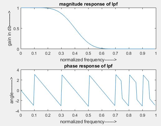
Program:
clc;
clear all;
close all;
n=20;
fp=200;
fq=300;
fs=1000;
fn=2*fp/fs;
window=blackman(n+1);
b=fir1(n,fn,window);
[H W]=freqz(b,1,128);
subplot(2,1,1);
plot(W/pi,abs(H));
title(‘magnitude response of lpf’);
ylabel(‘gain in db——–>’);
xlabel(‘normalized frequency——>’);
subplot(2,1,2);
plot(W/pi,angle(H));
title(‘phase response of lpf’);
ylabel(‘angle——–>’);
xlabel(‘normalized frequency——>’);
CHARACTER ORIENTED PROTOCOL AND BIT ORIENTED PROTOCOL
CHARACTER ORIENTED PROTOCOL:
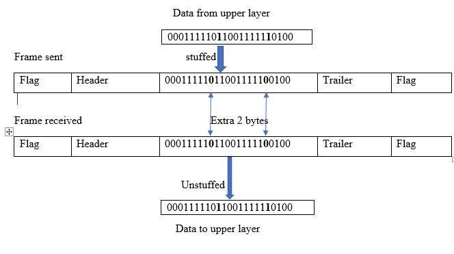
The character-oriented protocol is of an 8-bit size frame, the header which covers the source and destination address and some other control information, whereas the trailer carries error detection or error correction redundancy bits. In order to separate one frame from the next frame, the designer added a flag bit at the beginning and end of the frame. The most popular protocol which used to exchange only text by the data link layer.
If the receiver encounters other information rather than text in the middle of the data the user thinks of the end of the problem. To overcome this problem a byte-stuffing strategy was added to character-oriented framing. If the same pattern of the data found in the frame a special byte is added to the data section is called character stuffing (byte stuffing). This is called an escape character (ESC), which has a predetermined bit pattern. If we add ESC character in the middle of the data section means it treated has the next character as data, not a delimiting flag.
But it again creates a problem if the data contain an Escape character followed by a flag, by this the receiver will remove the ESC character from the data section but keeps the flag, which is incorrectly interpreted because of the end of the frame. To over the encountered problem, if the escape character is part of the text, an extra ESC character added to show that the second one is the part of the text.
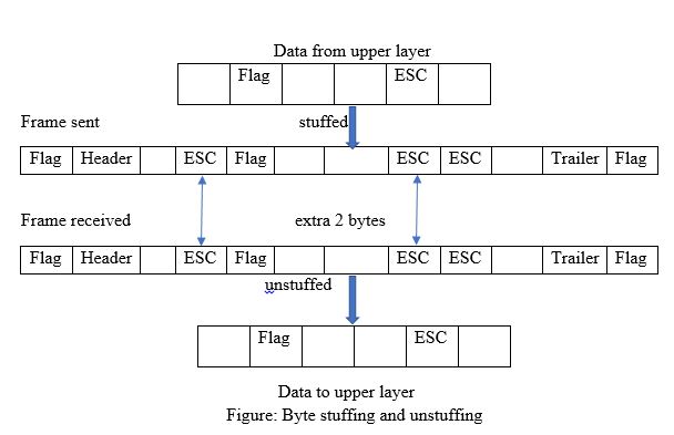
BIT ORIENTED PROTOCOL:
Bit stuffing is the process of adding one extra 0 whenever five consecutive is follow a 0 in the data so that the receiver does not mistake the pattern 0111110 for a flag. In this, the data section of a frame is a sequence of bits to be interpreted by the upper layer as text, audio, video, and audio, etc. Where in addition to the header, the designer will require a delimiter to separate one frame from other frames. Well, most protocols use a special 8-bit pattern flag as the delimiter to determine the starting and end of the frame.
Ethernet Standards
GIGABIT ETHERNET:
In order to provide higher order data rates it resulted in gigabit ethernet protocol. It standard is defined by IEEE as 802.3z. The main for designing gigabit ethernet is.
- It upgraded with the data rates upto 1 Gbps.
- It has same 48 bit address.
- Which has the same frame format compared with other standards.
In the full-duplex mode gigabit ethernet there is no collision; whereas the maximum length of the cable is determined by the signal attenuation in the cable.
Still there is use of half duplex in gigabit ethernet but it is rare. For this case the switch is replaced by hub.
While the physical layer is some complicated when compared with the traditional or standard methods. Let us discuss some features in the physical layer.
Gigabit is designed in such a way that we can connect two or more stations. If there is only one station it is connected in point-to-point. If their more than one station it is connected in a star topology with switch or hub at the center.
Gigabit ethernet can be categorized based on the wire implementation it may be two or four wire implementation. In two-wire implementation designer can use fiber-optic cable (100Base –SX, short wave, or 100 Base-LX, long range) or STP (shielded twisted pair)(1000 Base-CX)
. While in four-wire implementation designer can use category 5 twisted pair cable (1000 Base-T).
Gigabit ethernet using 8B/10B encoding scheme because Manchester encoding scheme involves high bandwidth. Where 8B/10B encoding scheme prevents long sequence of 0 or 1’s in the stream, but the resulting stream is 1.25 Gbps.
Where in four wire implementation it is not possible to use 2 wire for input and 2 wire for output, because each wire would need to carry 500 Mbps, which exceeds the category of 5 UTP to overcome the drawback designer used 4D-PAM5 encoding scheme to reduce the bandwidth.
Thus all, the four wire are involved in both input and output; while each wire carries 250Mbps, which is in the range of the category 5 UTP cable.
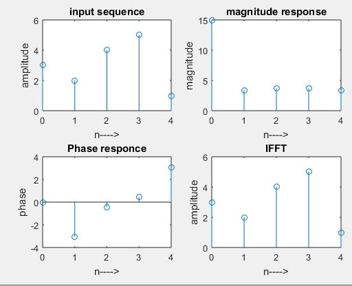
To Plot FFT (Fast Fourier Transform Algorithms) For the Given Sequence
Theory:
FFT is a most efficient algorithm used in speech processing, frequency estimation and communication. FFT utilizes full advantage of two symmetry properties in order to provide efficient algorithm for DFT. while considering a divide and conquer approach, a computationally efficient algorithm can be developed. This methods depends on the decomposition of an N-point DFT into successively smaller size then DFTs. While in the N-point sequence, the term N can be expressed as N = r1r2r3, …, rm, then N = r m, can be decimated into r-point sequences For each r point sequence, r-point DFT are often computed. Hence the DFT is of size r. if the number r is called the radix of the FFT algorithm while the number m indicates the number of stages in computation. If the value of r = 2, it is called radix-2 FFT.
Steps involved in finding the FFT of the given sequence:
- Let’s consider an input sequence as x[n].
- Let’s find the length for the input sequence using length command.
- In order to find FFT and IFFT by using the matlab commands fft and ifft.
- Let’s plot the magnitude and phase response for the given sequence.
- And finally display the results.
Program:
clc;
clear all;
close all;
x=input(‘Enter the sequence : ‘)
N=length(x)
xK=fft(x,N)
xn=ifft(xK)
n=0:N-1;
subplot (2,2,1);
stem(n,x);
xlabel(‘n—->’);
ylabel(‘amplitude’);
title(‘input sequence’);
subplot (2,2,2);
stem(n,abs(xK));
xlabel(‘n—->’);
ylabel(‘magnitude’);
title(‘magnitude response’);
subplot (2,2,3);
stem(n,angle(xK));
xlabel(‘n—->’);
ylabel(‘phase’);
title(‘Phase response’);
subplot (2,2,4);
stem(n,xn);
xlabel(‘n—->’);
ylabel(‘amplitude’);
title(‘IFFT’);
Output:
Enter the sequence: [3 2 4 5 1]
x = 3 2 4 5 1
N =5
xK =15.0000 + 0.0000i -3.3541 – 0.3633i 3.3541 – 1.5388i 3.3541 + 1.5388i -3.3541 + 0.3633i
xn =3.0000 2.0000 4.0000 5.0000 1.0000