• Data type specifies the type of data present inside a variable. • Every value has a data type • In python it is not required to specify the data type explicitly. • Based on the value, the type will be assigned automatically. • Python is dynamically typed language.
Python contains the following data types
• None • Numeric • List • Tuple • Set • String • Range • Dictionary/ mapping NONE: • If a variable is not assigned with any value is called None. Numeric • Numeric type of data is classified into four types
Int
Float
Complex
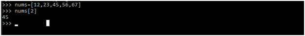
Bool Integer • Integer includes the values that are integers. • Integer type variables stores the values that are in integer format. • Example: num= 4 print(num) output :4 Float: • Float includes decimal numbers. Example • num= 5.5 print(num) output: 5.5 Complex: • It includes real and imaginary values. • Example:>>num=7+8j num= ‘7+8j’ print(num) output: 7+8j Note: In all the above data types we are not specifying the data type before the variable. This means that in python thee is no need to type the data type explicitly. It considers the type of the data based in the given input value
In order to compete with LAN protocols fast ethernet was designed.it can transmit data 10 times faster when compared with standard ethernet. It has 100mbps data rate, which has same minimum and maximum frame length when compared with standard ethernet. A new feature which added to fast ethernet is auto negotiation, which was designed particularly for the following uses.
It allows a device of 10 mbps is connected to a device of 100mbps capacity.
It allow one device to have multiple capabilities.
It also allowed to check the hub’s capabilities.
Fast ethernet was implemented at physical layer which is categorized has follows two-wire or four-wire. In two-wire implementation further categorized into 5 UTP (100Base-TX) or fiber-optic cable (100Base-Fx). And four-wire is implemented for 3 UTP (100 BaseT4).
The encoding scheme used for fast ethernet:
Manchester encoding scheme required 200-M baud bandwidth for the data rate of 100Mbps, which seems unsuitable for medium such as twisted-pair. For this reason, the fast ethernet was designed with an alternative encoding/decoding scheme.
100Base-TX:
It uses two pair of twisted-pair cable i.e., 5 UTP or STP. In order to obtain good performance and bandwidth MLT-3 scheme was implemented. Where MLT-3 scheme is not a self-synchronous line-coding scheme, for this we are providing 4B/5B block coding to provide bit synchronization by preventing the occurrence of a long sequence of 0s and 1s. Which will improves the data rate of 125 Mbps.
100Base-FX:
It uses two pair of twisted-pair of fiber-optic cables. This will handle high bandwidth requirement by using simple encoding schemes. In order to provide the above requirement designer provided NRZ-I encoding scheme which has a bit synchronization problem for long sequence of 0s.to over the above problem designer used 4B/5B encoding scheme which can improves the data rates from 100 to 125 mbps, which can be easily handled by fiber-optics.
100Base-T4: It was designed by using 3 or higher UTP. This implementation will be done by using four-pair of UTP for transmitting 100mbps. In this encoding/decoding schemes are more complicated, for this reason, the designer used three pairs of UTP category 3, however, can handle only 75 M baud each. In order to convert 100 Mbps to 75 M baud designer used 8B/6T to satisfies the above requirement.
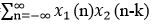
Auto Correlation Function Autocorrelation function is a measure of similarity between a signal & its time-delayed version. It is represented with R(k). While the autocorrelation function of x(n) is determined by
R11 (k) =R(k)=
Steps to perform auto correlation:
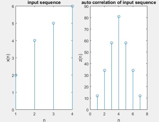
And the given input sequence is x[n].
Let the given impulse response of sequence h (n).
In order to auto correlation by using the matlab command xcorr.
Let’s plot the sequence x[n], h[n], z[n].
Next step is to display the result.
Program:
clc;
close all;
clear all;
% Let’s the two input sequences
x=input(‘enter input sequence’)
subplot(1,2,1);
stem(x);
xlabel(‘n’);
ylabel(‘x(n)’);
title(‘input sequence’);
% And the auto correlation of the given input sequence
The frequency response of the signal in differential equation form:
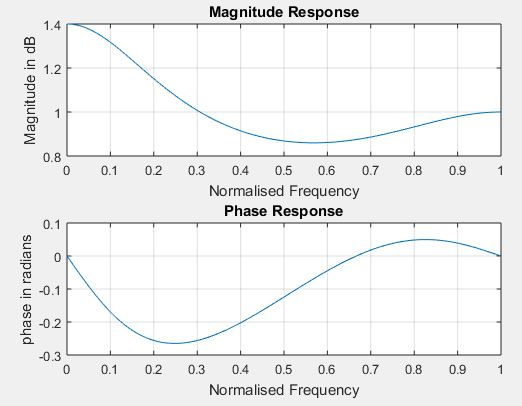
Systems respond differently to inputs of different frequencies. Where some of the systems may amplify components with certain frequencies, and attenuate components of other frequencies. And the way system output is related to the system input with different frequencies is called the frequency response of the system. We can convert it to polar notation in the complex plane. This will provides us the magnitude and an angle. We call the angle the phase.
Amplitude Response: For each frequency, the magnitude represents the system’s tendency to amplify or attenuate the input signal.
Phase Response: The phase represents the system’s tendency to modify the phase of the input sinusoids.
Steps for obtaining frequency response of the signal:
And the given numerator coefficients of the given transfer function or difference equation.
And the given denominator coefficients of the given transfer function or difference equation
Let’s pass these coefficients to matlab command freqz to find frequency response.
In order to find magnitude and phase response by using matlab commands abs and angle.
Depending on the encoding and decoding operation Ethernet are categorized into four:
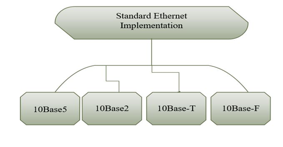
STANDARD ETHERNET:
Standard Ethernet is implemented using digital signaling with the data rates of 10 Mbps. Whereas at the sender, the data is converted into a digital signal using Manchester scheme. While at the receiver it uses Manchester scheme in order to decode the received signal. Manchester scheme is self-synchronous used for providing a transition at each bit interval. Standard Ethernet are categorized in to four types. They are as shown in below figure.
10BASE5 🙁 THICK ETHERNET)
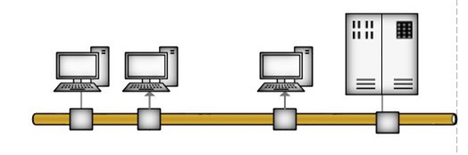
This is the first implementation of standard Ethernet it is also known as thick ethernet. Name is derived based on the size of the cable. It is the first implementation which used bus topology with an external transceiver connected via a tap to a thick coaxial cable. Where transceiver is used for transmitting and receiving and detecting collisions. In order to provide separate path for transmitting and receiving data via transceiver cable. The maximum length of the cable should not exceed 500m, otherwise there will be degradation of the signal.
Transceiver Thick coaxial cable maximum 500 m
10BASE2: (THIN ETHERNET)
Thin ethernet is the second implementation of standard ethernet it also uses the bus topology, but the cable very thinner and more flexible. In this, the transceiver is the part of the network interface card (NIC), which is installed inside the station. It is very less expensive when compared with the thick ethernet, Its installation is simpler because of flexible. And the length of the thin ethernet is 185m.
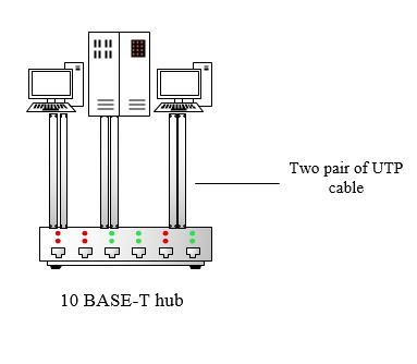
10BASE-T: (TWISTED PAIR)
Twisted pair ethernet is the third implementation of the standard ethernet, which uses star topology. In which stations are connected to a hub via two pair of twisted cable. In this two pair of twisted cable create two paths between the station and hub. The maximum length of the cable is 100m.
10BASE-F: (FIBER CABLE)
10BASE-F uses a star topology to connect stations to a hub, the stations are connected to the hub using two fiber-optics cables.
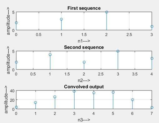
Convolution is a mathematical way of combining the two signals to form a third signal. It is the only most vital technique in Digital Signal Processing. Using the strategy of impulse decomposition, systems are described by a sign called the impulse response. Convolution is vital because it relates the three signals of interest: the input, the output, and therefore the impulse response. When convolution is used with linear systems. An input, x[n], enters a linear system with an impulse response, h[n], leading to an output, y[n].In equation form: x[n] * h[n] = y[n]. Expressed in words, the input convolved with the impulse response is adequate to the output. Just as addition is represented by the plus, +, and multiplication by the cross, x, convolution is represented by the star, *. The equation represents the linear convolution equation. Zero-padding is used in correlation to avoid mixing of convolution results at the output (due to circular convolution).
x[n] *h[n] = y[n]
Steps for performing linear operation:
Give input sequence x[n].
Give impulse response sequence h (n):
Find the convolution y[n] using the matlab command conv.