linear Convolution Theory:
Convolution is a mathematical way of combining the two signals to form a third signal. It is the only most vital technique in Digital Signal Processing. Using the strategy of impulse decomposition, systems are described by a sign called the impulse response. Convolution is vital because it relates the three signals of interest: the input, the output, and therefore the impulse response. When convolution is used with linear systems. An input, x[n], enters a linear system with an impulse response, h[n], leading to an output, y[n].In equation form: x[n] * h[n] = y[n]. Expressed in words, the input convolved with the impulse response is adequate to the output. Just as addition is represented by the plus, +, and multiplication by the cross, x, convolution is represented by the star, *. The equation represents the linear convolution equation. Zero-padding is used in correlation to avoid mixing of convolution results at the output (due to circular convolution).
x[n] *h[n] = y[n]
Steps for performing linear operation:
- Give input sequence x[n].
- Give impulse response sequence h (n):
- Find the convolution y[n] using the matlab command conv.
- Plot x[n],h[n],y[n].
Program:
clc;
clear all;
close all;
x1=input(‘Enter the first sequence x1(n) = ‘);
x2=input(‘Enter the second sequence x2(n) = ‘);
L=length(x1);
M=length(x2);
N=L+M-1;
yn=conv(x1,x2);
disp(‘The values of yn are= ‘);
disp(yn);
n1=0:L-1;
subplot(311);
stem(n1,x1);
grid on;
xlabel(‘n1—>’);
ylabel(‘amplitude—>’);
title(‘First sequence’);
n2=0:M-1;
subplot(312);
stem(n2,x2);
grid on;
xlabel(‘n2—>’);
ylabel(‘amplitude—>’);
title(‘Second sequence’);
n3=0:N-1;
subplot(313);
stem(n3,yn);
grid on;
xlabel(‘n3—>’);
ylabel(‘amplitude—>’);
title(‘Convolved output’);
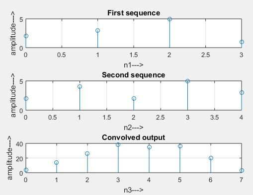
Output:
Enter the first sequence x1(n) = [2 3 5 1]
Enter the second sequence x2(n) = [2 4 2 5 3]
The values of yn are=
4 14 26 38 35 36 20 3