Convolution for both signals and sequence:
Convolution is defined as mathematical way of combining two signals in order to form third the signal. It plays a significant role because it relates the input signal and impulse response of the system to the output of the system. Which is used to provide relationship of LTI system.
Some important properties of convolution are:
Let us consider two signals x1(t) and x2(t) for these the convolution is
x1(t)* x2(t) = ) ) = ) )
Commutative property:
The commutative property of convolution is
x1(t)*x2(t) = x2(t) *x1(t)
Distributive property:
The Distributive property of convolution is
x1(t)*[ x2(t)+ x3(t)]= [x1(t)* x2(t)]+[ x1(t)* x3(t)]
Associative property:
The Associative property of convolution is
x1(t)*[ x2(t)*x3(t)]= [x1(t)* x2(t)]* x3(t)
Convolution performs the following operations are:
- Folding
- Multiplication
- Addition
- Shifting
clc;
close all;
clear all;
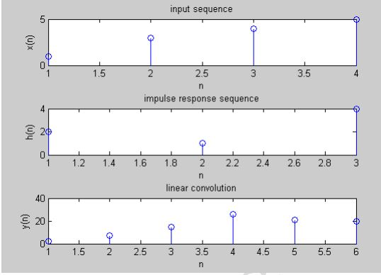
%program for convolution of two sequences
x=input(‘enter input sequence: ‘);
h=input(‘enter impulse response: ‘);
y=conv(x,h);
subplot(3,1,1);
stem(x);
xlabel(‘n’);
ylabel(‘x(n)’);
title(‘input sequence’)
subplot(3,1,2);
stem(h);
xlabel(‘n’);
ylabel(‘h(n)’);
title(‘impulse response sequence’)
subplot(3,1,3);
stem(y);
xlabel(‘n’);
ylabel(‘y(n)’);
title(‘linear convolution’)
disp(‘linear convolution y=’);
disp(y)
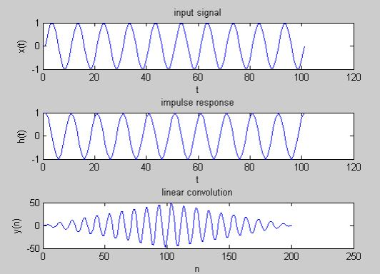
%program for signal convolution
t=0:0.1:10;
x1=sin(2*pi*t);
h1=cos(2*pi*t);
y1=conv(x1,h1);
figure;
subplot(3,1,1);
plot(x1);
xlabel(‘t’);
ylabel(‘x(t)’);
title(‘input signal’)
subplot(3,1,2);
plot(h1);
xlabel(‘t’);
ylabel(‘h(t)’);
title(‘impulse response’)
subplot(3,1,3);
plot(y1);
xlabel(‘n’);
ylabel(‘y(n)’);
title(‘linear convolution’);