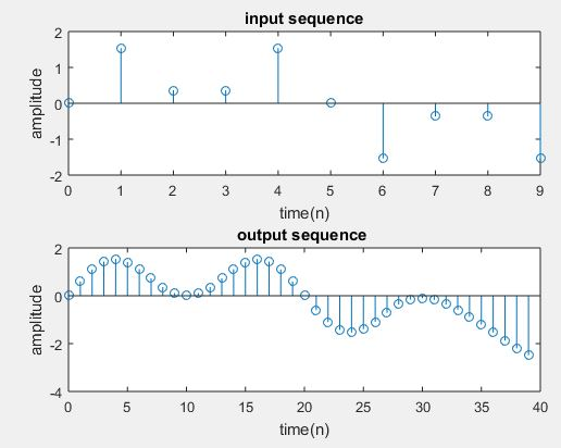
Interpolation Process Implementation:
Theory:
“Upsampling” is defined as the process of inserting zero-valued samples between original samples to increase the sampling rate. (This is called “zero-stuffing”.) . “Interpolation”, is determined as the process of upsampling followed by filtering. The filtering removes the undesired spectral images. The main reason for interpolating is simply used to maximize the sampling rate at the output of a particular system so that another system operating at a better rate can input the signal.
Steps to perform interpolation process:
Step I: Let’s define up sampling factor and input frequencies f1 and f2
Step II: Now represents the input sequence with frequencies f1 and f2
Step III: In order to perform the interpolation on input signal by using the matlab command interp.
Step IV: Next to plot the input and output signal/sequence.
Program:
clc;
clear all;
close all;
L=input(‘enter the upsampling factor’);
N=input(‘enter the length of the input signal’); % its Length should be always greater than 8
f1=input(‘enter the frequency of first sinusoidal’);
f2=input(‘enter the frequency of second sinusoidal’);
n=0:N-1;
x=sin(2*pi*f1*n)+sin(2*pi*f2*n);
y=interp(x,L);
subplot(2,1,1)
stem(n,x(1:N))
title(‘input sequence’);
xlabel(‘time(n)’);
ylabel(‘amplitude’);
subplot(2,1,2)
m=0:N*L-1;
stem(m,y(1:N*L))
title(‘output sequence ‘);
xlabel(‘time(n)’);
ylabel(‘amplitude’);
Output:
enter the upsampling factor4
enter the length of the input signal10
enter the frequency of first sinusodal0.1
enter the frequency of second sinusodal0.3
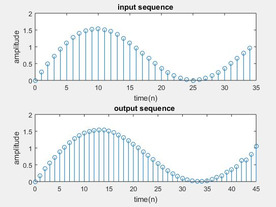
I/D sampling rate convertor implementation:
Steps to perform the I/D sampling rate conversion:
Step I: Let’s define the upsampling factor, downsampling, and input frequencies f1 and
f2
Step II: Let’s represent the input sequence with frequencies f1 and f2
Step III: In order to perform I/D sampling rate conversion on the given input signal by using Matlab resample.
Step IV: To plot the input and output signal/sequence.
Program:
clc;
clear all;
close all;
L=input(‘enter the upsampling factor’);
D=input(‘enter the downsampling factor’);
N=input(‘enter the length of the input signal’);
f1=input(‘enter the frequency of first sinusoidal’);
f2=input(‘enter the frequency of second sinusoidal’);
n=0:N-1;
x=sin(2*pi*f1*n)+sin(2*pi*f2*n);
y=resample(x,L,D);
subplot(2,1,1)
stem(n,x(1:N))
title(‘input sequence’);
xlabel(‘time(n)’);
ylabel(‘amplitude’);
subplot(2,1,2)
m=0:N*L/D-1;
stem(m,y(1:N*L/D));
title(‘output sequence ‘);
xlabel(‘time(n)’);
ylabel(‘amplitude’);
output:
enter the upsampling factor4
enter the downsampling factor3
enter the length of the input signal35
enter the frequency of first sinusodal0.01
enter the frequency of second sinusodal0.03