Thursday, March 5, 2026
Home Blog Page 8

How to check the keywords in python? Syntax for python and Different ways of running python script

0

How to check the keywords in python?

The number of keywords in python changes frequently. In some cases keywords are converted to     built -in functions. for example exec and print were the keywords in python 2.7 but in python 3 + they are converted as built in functions.

To check the list of  keywords in python  type

Help(“keywords”)

Then it will display the list of keywords in python.

Syntax for python

  • Syntax for any programming language is the set of rules that defines how a program should be written  and interpreted.
  • In python we can type the code in the command line prompt and execute  directly.

Different ways of running python script

There are different ways of running python script

Interactive Mode

  • One of the most widely used way of running python script  is interactive mode.   
  • To execute the code in interactive mode  simply go to command prompt and type python .Then it will display the information of python version installed in your pc.
  • Next, type the code and hit enter.

Example:

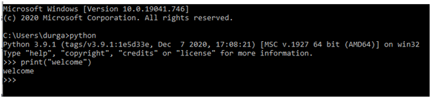
Here in the above the print function is used to print the text whatever inside the parenthesis.

Here  we are entering the text  that means it is in string format so it should be mentioned either  in single quote or double quote.

Example 2:

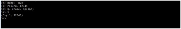
You can run more than two lines code in interactive mode.

Note:  To get out of this mode  press ctrl +Z  or  type exit() and press enter.
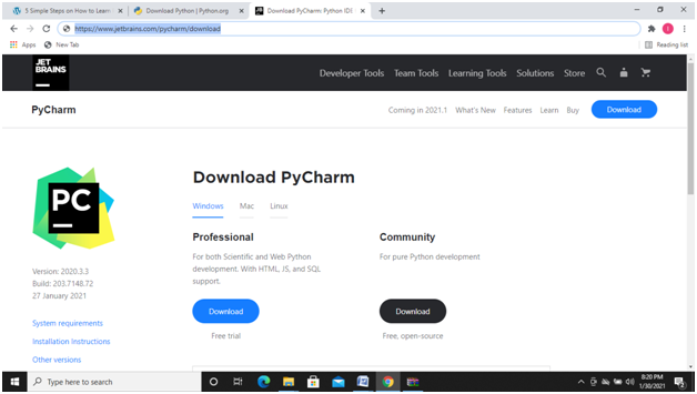
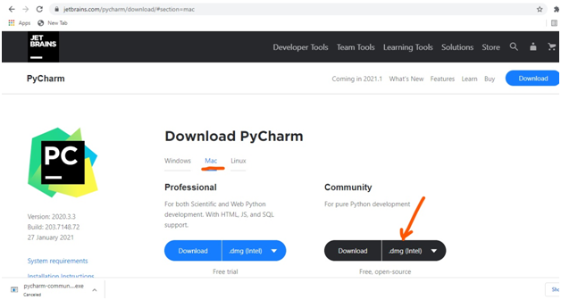
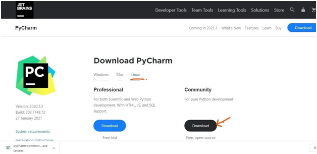
PyCharm IDE

Torun the python code using an IDE like  PyCharm. The following steps should be followed.

  1. Install PyCharm IDE and set environment path variable.
  2. Open the Pycharm IDE.
  3. Create a new project
  4. Specify a name to the project.
  5. Write the code and run.
  6. Code is executed.

Note:  The advantage of using interpreter like Py Charm is that the file is not required  to save with .py extension. It automatically saved with .py extension

To Plot the DFT/IDFT for the Given Discrete Signal

0

Theory:

Frequency analysis of discrete time signals is usually performed on digital signal processor, which may be general purpose digital computer or specially designed digital hardware. To perform frequency analysis on discrete time signal, we convert the time domain sequence to an equivalent frequency domain representation. We know that such representation is given by The Fourier transform X(ejw) of the sequence x(n). However, X(ejw) is a continuous function of frequency and therefore, It is not a computationally convenient representation of the sequence. DFT is a powerful computational tool for performing frequency analysis of discrete time signals. The N-point DFT of discrete time sequence x(n) is denoted by X(k) and is defined as.

x(n)= n)

Steps in performing operations:

  • Get the input sequence.
  • We can find the DFT for the input sequence using by direct equation of DFT.
  • Find the IDFT using the direct equation.
  • Let’s plot the DFT and IDFT for the given sequence by using matlab command stem.
  • Display the above outputs.

Program:

clc;

close all;

clear all;

xn=input(‘Enter the sequence x(n)’);

ln=length(xn); %find the length of the sequence

xk=zeros(1,ln); %let’s initialize an array of the same size as that of input sequence

ixk=zeros(1,ln); let’s initialize an array of the same size as that of input sequence

%DFT of the sequence

for k=0:ln-1

 for n=0:ln-1

 xk(k+1)=xk(k+1)+(xn(n+1)*exp((i)*2*pi*k*n/ln));

 end

end

%Plotting input sequence

t=0:ln-1;

subplot(221);

stem(t,xn);

ylabel (‘Amplitude’);

xlabel (‘Time Index’);

title(‘Input Sequence’);

magnitude=abs(xk); % In order to find the magnitudes for the individual DFT points

% plot the magnitude response

t=0:ln-1;

subplot(222);

stem(t,magnitude);

ylabel (‘Amplitude’);

xlabel (‘K’);

title(‘Magnitude Response’);

phase=angle(xk); % In order to find the phases of individual DFT points % plot the magnitude

t=0:ln-1;

subplot(223);

stem(t,phase);

ylabel (‘Phase’);

xlabel (‘K’);

title (‘Phase Response’);

%IDFT of the sequence

for n=0:ln-1

 for k=0:ln-1

 ixk(n+1)=ixk(n+1)+(xk(k+1)*exp(i*2*pi*k*n/ln));

 end

end

ixk=ixk./ln;

%code block to plot the input sequence

t=0:ln-1;

subplot(224);

stem(t,ixk);

ylabel (‘Amplitude’);

xlabel (‘Time Index’);

title (‘IDFT sequence’);

Requirement Of Flow Control and Error control

Importance Of Flow And Error Control:

The most important function of the data link layer is to provide flow control and error control mechanisms. In data communication it requires, when two devices working together, one device for sending and other for receiving for correcting errors.

Flow control:

The most important duty of data link layer is flow control coordinates the amount of data can be sent before receiving acknowledgement.

From most protocols, flow control is a set of procedures that tells the sender how much data it can transmit before it must wait for an acknowledgement from the receiver,

Any receiving device has a limited speed at which it can process incoming data and a limited amount of memory in which to store incoming data, the receiving devices must be ready to inform the sending device before those limits are reached and to request that the transmitting device send fewer frames or stop temporarily.

Incoming data must be checked and processed before they will be used. The rate of such processing is usually slower than the speed of transmission. For this reason, each receiving device features a block of memory, called a buffer, reserved for storing incoming data until they’re processed. If the buffer begins to refill, the receiver must be ready to tell the sender to halt transmission until it’s once more ready to receive.

Error control:


Error control is used for the both error detection and error correction. It allows the receiver to tell the sender of any frames lost or damaged in transmission and coordinates the retransmission of these frames by the sender.
The term error control refers primarily to methods of error detection and retransmission in the data link layer.
Anytime a mistake is detected in an exchange, specified frames are retransmitted. This process is called automatic repeat request (ARQ).

Keywords in python

0

  • In python there are some reserved words called as keywords, These keywords are used for writing syntax and for some special purposes these are used for that particular purposes only.  and are not allowed to use as variable name ,identifier and function names.
  • One thing to note is that these key words are different from built in functions. Built in functions are not as restricted as keywords.
  • An example to demonstrate the difference between the built in function and keywords is you  can be able to assign something  to built-in function where as for keywords it is not possible. But assigning something to built in function is not good practice.
  • These keywords are case sensitive.
  • All these keywords except True , False and None are case sensitive.

The following is the list of keywords in python

 andcontinuefinallyimportraise
 asdefforlambdareturn
 assertdelfromNoneTrue
asyncelifglobalnotTry
awaitelseinnormalWith
breakexceptiforWhile
classFalseispassYield

Ethernet Frame Format

Ieee 802.3 Frame Format(Ethernet):

The ethernet frame format has seven filelds :preamble,start frame delimiter(SFD), destination address(DA),source address(SA),length or type,data, cyclic redundancy check(CRC). In ethernet their no acknownledgement mechanism in order to intemate received frame,well acknowledgement is implemented in higher layers.

  Preamble (7 bytes)SFD (1bytes) Destination Address (6 bytes)Source address (6 bytes)Length or type (2 bytes)Data and              padding  CRC (4 bytes)

Fig: frame format of ieee 802.3

Preamble:

It is the first field in the ethernet frame format which contains 7 bytes of alternating 0 and 1 that informs the receiving system to the coming frame and enables it to synchronize its input timing.this is actually added at the physical layer and is not part of the frame.

Start Frame Delimiter:

It is the second filed in the Ethernet frame format which contains 1 byte. It determines the beginning of the frame. SFD warns the stations or station about the chance for synchronization.

Destination Address:

This field has 6 bytes which contains the physical address of the destination station or stations to receive the packet.

Source Address:

This field has 6 bytes which contains the physical address of the sender of the packet.

Length or type:

This filed is defined as a type or length field. The original Ethernet used this field because the type filed to define the upper-layer protocol using the MAC frame. The IEEE standard used as the length filed to define the number of bytes in the data field. It is of 2 bytes field.

Data:

This field carries data encapulsated from the upper layer protocal. It is a minimum of 46 bytes andmaximum of 1500 bytes.

CRC:

This is of 4 bytes field used for error detection.

Data field:

Destination Address (6 bytes)Source address (6 bytes)Length or type (2 bytes)Data and              padding  CRC (4 bytes)

                                                                       Minimum payload length:46 bytes

                                                                     Maximum payload length:1500 bytes

The Minimum frame length has: 512 bits or 64 bytes

The Maximum frame length has:12,144 bits or 1518 bytes

Fig: Minimum and maximum lengths

Addressing:

Each station on ethernet network conisting of its own network interface card(NIC). NIC is fixed inside the station and provides the station with a 6 bytes physical address. Let consider an example of ethernet in hexadecimal notation.

06:01:02:01:2C:4B

6 bytes =12 hex digits =48 bits

Unicast, multicast and broadcast address:

The least significant bit(LSB) of the first byte will defines the type of address. If the bit is determined as 0, the address is unicast otherwise it is defined as multicast.

The broadcast destination address is a special case of the multicast address in which all its are 1s.

Let us consider  an example in order to define destination address.

4A:30:10:21:01:1A

To find the type of address, we need to look at the second hexadecimal digit from the left.if it even the address is unicast. If it is odd the address is multicast.if all the digits are F’s the address is broadcast.

Given example is unicast address because A in binary is 1010(even)

47:20:1B:2E:08:EE

Given example is multicast address because 7 in binary is 0111(odd)

Wiener-Khinchin theorem verification

0

Wiener-Khinchin:

The Wiener-Khinchin theorem is a fundamental theorem useful for the stochastic processes. The Wiener-Khinchin theorem provides a simple relationship between time and frequency representations of a fluctuating process. Its great practical importance comes from the fact that the autocorrelation function may be directly determined from the measured power spectral density, and vice versa. The wiener-Khinchin is widely used theorem to states the power spectral density of a wide sense stationary random process of the flourier transform for the corresponding autocorrelation function.

Program:

clc;

clear all;

close all;

t=0:0.1:2*pi;

%input signal

x=sin(2*t);

subplot(3,1,1);

plot(x);

xlabel(‘time’);

ylabel(‘amplitude’);

title(‘input signal’);

%autocorrelation of input signal

xu=xcorr(x,x);

%fft of autocorrelation signal

y=fft(xu);

subplot(3,1,2);

plot(abs(y));

xlabel(‘f’);

ylabel(‘amplitude’);

title(‘fft of autocorrelation of input signal’);

%fourier transform of input signal

y1=fft(x);

%finding the power spectral density

y2=(abs(y1)).^2;

subplot(3,1,3);

plot(y2);

xlabel(‘f’);

ylabel(‘magnitude’);

title(‘PSD of input signal’);

Extraction Of Periodic Signal Using Correlation:

A signal is masked by noise are often detected either by correlation techniques or by filtering. Actually, the two techniques are equivalent. The correlation technique may be a measure of extraction of a given signal within the time domain whereas filtering achieves precisely the same leads to frequency domain.

Program:

clear all;

close all;

clc;

t=0:0.1: pi*4;

%input signal1

s=sin(t);

subplot(7,1,1)

plot(s);

title(‘signal s’);

xlabel(‘t’);

ylabel(‘amplitude’);

%input signal2

c=cos(t);

subplot(7,1,2)

plot(c);

title(‘signal c’);

xlabel(‘t’);

ylabel(‘amplitude’);

%generating noise signal

n = randn([1 126]);

%signal+noise

f=s+n;

subplot(7,1,3);

plot(f);

title(‘signal f=s+n’);

xlabel(‘t’);

ylabel(‘amplitude’);

%cross correlation of signal1&signal2

asc=xcorr(s,c);

subplot(7,1,4)

plot(asc);

title(‘ correlation of s and c’);

xlabel(‘t’);

ylabel(‘amplitude’);

%cross correlation of noise&signal2

anc=xcorr(n,c);

subplot(7,1,5)

plot(anc);

title(‘ correlation of n and c’);

xlabel(‘t’);

ylabel(‘amplitude’);

%cross correlation of f&signal2

cfc=xcorr(f,c);

subplot(7,1,6)

plot(cfc);

title(‘ correlation of f and c’);

xlabel(‘t’);

ylabel(‘amplitude’);

%extracting periodic signal

hh=asc+anc;

subplot(7,1,7)

plot(hh);

title(‘addition of sc+nc’);

xlabel(‘t’);

ylabel(‘amplitude’);

Installation of PyCharm IDE for Mac, Windows and Linux

0

Installation of PyCharm IDE

  1. Navigate to official Pycharm websitehttps://www.jetbrains.com/pycharm..\Downloads\latest and download Pycharm .
  2.  Run the exe file to Install PyCharm  and you can also install PyCharm on windows manually by configuring PyCharm location on your c drive or change location of PyCharm .
  3. You can effortlessly configure PyCharm on windows 10 and to code in python you need to install PyCharm in windows 10 depending up on your system compatibility if its 32 but 0r 64 bit.
  4.  PyCharm is not only the IDE through which you can execute python code in windows 10 but    PyCharm is the most widely used IDE or integrated development environment for Python & compatable and will execute complex python code easily. 
  5. PyCharm  is accesable in three editions  ProfessionalCommunity, and Edu. It offers to download in 32 bit and 62 bit for windows 10 and also you can install pycharm on your mac by downloading .dmg file.

How to install Pycharm on Windows

The following is the step by step procedure to install Pycharm in windows 10

  1. To download and install Pycharm go to the official website https://www.jetbrains.com/pycharm.
  2. Download the community version

Install the downloaded file.

How to install Pycharm in Mac?

The following is the step by step procedure to install Pycharm for Mac

  1. Navigate to the official website and download the .dmg file.
  2. Install the downloaded file.

How to install Pycharm in Linux?

1. Go to the official website of Pycharm

2.  click on the Linux OS and download.

3. Install the downloaded file.

Installation of Python for Mac and Windows OS

0

How to install python

  1. Open the official website of python  i.e., https://www.python.org
  2. Go to downloads https://www.python.org/downloads
  1. Download the latest version of python depending on your OS.
  2. Install the downloaded file.

 Downloading Python for Mac OS

  1. Open the official website of Python and click on the type of OS and download the latest release.
  2. Install the downloaded file.

Downloading Python for Windows

  1. Go to official website of python as suggested above and click on windows OS and download the latest release.
  2. Install the  downloaded file.

Introduction, uses and features of Python programming

0

What is python programming?

  • Python is a high level dynamically typed and interpreted object oriented high level programming language
  • Though there are many programming languages  in the market like C, C++,  java, java script python has its own popularity.
  • Though python came into light before java but it has not acquired the identification that it has today.  Python was developed by Guido Van Rossum and released in 1991.
  •   But for beginners of programming the programming language must be easier to understand python is such easiest language to learn..
  •  With the development of machine learning, Python has grasped more attention for  researchers as it is the easiest language for programming.

Use of python Programming?

  • Python  programming is used to create web applications.
  • Python programming is used to create workflows.
  • Python programming  is used for production ready software development and  rapid prototyping.
  • Python programming is capable of handling big data and also performs complex mathematical computations.
  • With the python programming one can connect to database systems.
  • Python can also be capable of reading and modifying the files.

Features of python:

Easy to use:

Python is easy to use and learn .It has simple structure, understandable syntax and developer friendly.

Multi-platform language:

Python can run on any platform such as Linux, windows, Unix etc.,

Open source software:

Python is an open source software available to everyone.

GUI programming:

Python is used for developing GUI(Graphical User Interface) applications.

Extensible:

This means that low level languages like C, C++, can be used to compile the code.

Integrated:

Python can be easily integrated with other languages like C, C++ Java.

Wide Frameworks and Libraries:

Python has wide range of libraries and frameworks for application developments.

Object oriented:

Python is an Object Oriented Programming language with classes and object concepts.

Sampling Theorem Verification, Noise removal by using cross-correlation/autocorrelation

0

Sampling theorem:

Sampling theorem is used to convert analog signal into discrete time signal.it has applications in digital signal processing and digital communication. Sampling theorem is determined has that if the sampling rate in any pulse modulation system exceeds twice the maximum frequency of the message signal, with this the receiver will reconstructed the signal with minimum distortion.

Whereas,

 fs is the sampling rate

fm is the maximum frequency of message signal

Then sampling theorem can be expressed in mathematical form as

Fs≥ 2fm

Well 2fm is determined as Nyquist rate.

It the condition is

Fs≤2fm

It is defined as aliasing effect it occurred when the sampling rate is less than twice the maximum frequency of the message signal.

Fs=sampling rate

Program:

clc;

clear all;

close all;

t=-10:.01:10;

T=4;

fm=1/T;

x=cos(2*pi*fm*t);

subplot(2,2,1);

plot(t,x);

xlabel(‘time’);

ylabel(‘x(t)’);

title(‘continous time signal’);

grid;

n1=-4:1:4;

fs1=1.6*fm;

fs2=2*fm;

fs3=8*fm;

x1=cos(2*pi*fm/fs1*n1);

subplot(2,2,2);

stem(n1,x1);

xlabel(‘time’);

ylabel(‘x(n)’);

title(‘discrete time signal with fs<2fm’);

hold on;

subplot(2,2,2);

plot(n1,x1);

grid;

n2=-5:1:5;

x2=cos(2*pi*fm/fs2*n2);

subplot(2,2,3);

stem(n2,x2);

xlabel(‘time’);

ylabel(‘x(n)’);

title(‘discrete time signal with fs=2fm’);

hold on;

subplot(2,2,3);

plot(n2,x2)

grid;

n3=-20:1:20;

x3=cos(2*pi*fm/fs3*n3);

subplot(2,2,4);

stem(n3,x3);

xlabel(‘time’);

ylabel(‘x(n)’);

title(‘discrete time signal with fs>2fm’)

hold on;

subplot(2,2,4);

plot(n3,x3)

grid;

Noise removal by using cross-correlation/autocorrelation

Detection of the periodic signal conceal by random noise is of great importance .The noise signal encountered in practice may be a signal with random amplitude variations. A signal is uncorrelated with any periodic signal. If s(t) is a periodic signal and n(t) is a noise signal then.

clc;

clear all;

close all;

t=0:0.2:pi*8;

%input signal

s=sin(t);

subplot(6,1,1);

plot(s);

title(‘signal s’);

xlabel(‘t’);

ylabel(‘amplitude’);

%generating noise

n = randn([1 126]);

%noisy signal

f=s+n;

subplot(6,1,2)

plot(f);

title(‘signal f=s+n’);

xlabel(‘t’);

ylabel(‘amplitude’);

%autocorrelation of input signal

as=xcorr(s,s);

subplot(6,1,3);

plot(as);

title(‘auto correlation of s’);

xlabel(‘t’);

ylabel(‘amplitude’);

%autocorrelation of noise signal

an=xcorr(n,n);

subplot(6,1,4)

plot(an);

title(‘auto correlation of n’);

xlabel(‘t’);

ylabel(‘amplitude’);

%autocorrelation of transmitted signal

cff=xcorr(f,f);

subplot(6,1,5)

plot(cff);

title(‘auto correlation of f’);

xlabel(‘t’);

ylabel(‘amplitude’);

%autocorrelation of received signal

hh=as+an;

subplot(6,1,6)

plot(hh);

title(‘addition of as+an’);

xlabel(‘t’);

ylabel(‘amplitude’);